Introduction to Numpy 
Sign up to the DEA Sandbox to run this notebook interactively from a browser
Compatibility: Notebook currently compatible with both the
NCIandDEA SandboxenvironmentsPrerequisites: Users of this notebook should have a basic understanding of:
How to run a Jupyter notebook
Background
Numpy is a Python library which adds support for large, multi-dimension arrays and metrics, along with a large collection of high-level mathematical functions to operate on these arrays. More information about numpy arrays can be found here.
Description
This notebook is designed to introduce users to numpy arrays using Python code in Jupyter Notebooks via JupyterLab.
Topics covered include:
How to use
numpyfunctions in a Jupyter Notebook cellUsing indexing to explore multi-dimensional
numpyarray dataNumpydata types, broadcasting and booleansUsing
matplotlibto plotnumpydata
Getting started
To run this notebook, run all the cells in the notebook starting with the “Load packages” cell. For help with running notebook cells, refer back to the Jupyter Notebooks notebook.
Load packages
In order to be able to use numpy we need to import the library using the special word import. Also, to avoid typing numpy every time we want to use one if its functions we can provide an alias using the special word as:
[1]:
import numpy as np
Introduction to Numpy
Now, we have access to all the functions available in numpy by typing np.name_of_function. For example, the equivalent of 1 + 1 in Python can be done in numpy:
[2]:
np.add(1, 1)
[2]:
2
Although this might not at first seem very useful, even simple operations like this one can be much quicker in numpy than in standard Python when using lots of numbers (large arrays).
To access the documentation explaining how a function is used, its input parameters and output format we can press Shift+Tab after the function name. Try this in the cell below
[3]:
np.add
[3]:
<ufunc 'add'>
By default the result of a function or operation is shown underneath the cell containing the code. If we want to reuse this result for a later operation we can assign it to a variable:
[4]:
a = np.add(2, 3)
The contents of this variable can be displayed at any moment by typing the variable name in a new cell:
[5]:
a
[5]:
5
Numpy arrays
The core concept in numpy is the “array” which is equivalent to lists of numbers but can be multidimensional. To declare a numpy array we do:
[6]:
np.array([1, 2, 3, 4, 5, 6, 7, 8, 9])
[6]:
array([1, 2, 3, 4, 5, 6, 7, 8, 9])
Most of the functions and operations defined in numpy can be applied to arrays. For example, with the previous operation:
[7]:
arr1 = np.array([1, 2, 3, 4])
arr2 = np.array([3, 4, 5, 6])

np.add(arr1, arr2)
[7]:
array([ 4, 6, 8, 10])
But a more simple and convenient notation can also be used:
[8]:
arr1 + arr2
[8]:
array([ 4, 6, 8, 10])
Indexing
Arrays can be sliced and diced. We can get subsets of the arrays using the indexing notation which is [start:end:stride]. Let’s see what this means:
[9]:
arr = np.array([0, 1, 2, 3, 4, 5, 6, 7, 8, 9, 10, 11, 12, 13, 14, 15])

print("6th element in the array:", arr[5])
print("6th element to the end of array", arr[5:])
print("start of array to the 5th element", arr[:5])
print("every second element", arr[::2])
6th element in the array: 5
6th element to the end of array [ 5  6  7  8  9 10 11 12 13 14 15]
start of array to the 5th element [0 1 2 3 4]
every second element [ 0  2  4  6  8 10 12 14]
Try experimenting with the indices to understand the meaning of start, end and stride. What happens if you don’t specify a start? What value does numpy uses instead? Note that numpy indexes start on 0, the same convention used in Python lists.
Indexes can also be negative, meaning that you start counting from the end. For example, to select the last 2 elements in an array we can do:
[10]:
arr[-2:]
[10]:
array([14, 15])
Multi-dimensional arrays
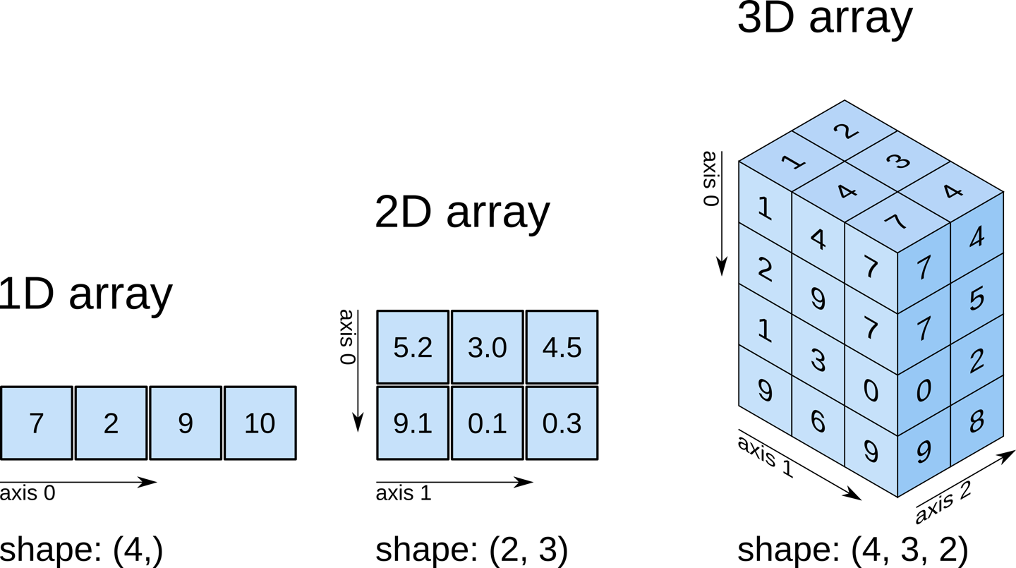
Numpy arrays can have multiple dimensions. For example, we define a 2-dimensional (1,9) array using nested square bracket:
[11]:
np.array([[1, 2, 3, 4, 5, 6, 7, 8, 9]])
[11]:
array([[1, 2, 3, 4, 5, 6, 7, 8, 9]])
To visualise the shape or dimensions of a numpy array we can add the suffix .shape
[12]:
print(np.array([1, 2, 3, 4, 5, 6, 7, 8, 9]).shape)
print(np.array([[1, 2, 3, 4, 5, 6, 7, 8, 9]]).shape)
print(np.array([[1], [2], [3], [4], [5], [6], [7], [8], [9]]).shape)
(9,)
(1, 9)
(9, 1)
Any array can be reshaped into different shapes using the function reshape:
[13]:
np.array([1, 2, 3, 4, 5, 6, 7, 8]).reshape((2, 4))
[13]:
array([[1, 2, 3, 4],
       [5, 6, 7, 8]])
If you are concerned about having to type so many squared brackets, there are more simple and convenient ways of doing the same:
[14]:
print(np.array([1, 2, 3, 4, 5, 6, 7, 8, 9]).reshape(1, 9).shape)
print(np.array([1, 2, 3, 4, 5, 6, 7, 8, 9]).reshape(9, 1).shape)
print(np.array([1, 2, 3, 4, 5, 6, 7, 8, 9]).reshape(3, 3).shape)
(1, 9)
(9, 1)
(3, 3)
Also there are shortcuts for declaring common arrays without having to type all their elements:
[15]:
print(np.arange(9))
print(np.ones((3, 3)))
print(np.zeros((2, 2, 2)))
[0 1 2 3 4 5 6 7 8]
[[1. 1. 1.]
 [1. 1. 1.]
 [1. 1. 1.]]
[[[0. 0.]
  [0. 0.]]

 [[0. 0.]
  [0. 0.]]]
Arithmetic operations
Numpy has many useful arithmetic functions. Below we demonstrate a few of these, such as mean, standard deviation and sum of the elements of an array. These operation can be performed either across the entire array, or across a specified dimension.
[16]:
arr = np.arange(9).reshape((3, 3))
print(arr)
[[0 1 2]
 [3 4 5]
 [6 7 8]]
[17]:
print("Mean of all elements in the array:", np.mean(arr))
print("Std dev of all elements in the array:", np.std(arr))
print("Sum of all elements in the array:", np.sum(arr))
Mean of all elements in the array: 4.0
Std dev of all elements in the array: 2.581988897471611
Sum of all elements in the array: 36
[18]:
print("Mean of elements in array axis 0:", np.mean(arr, axis=0))
print("Mean of elements in array axis 1:", np.mean(arr, axis=1))
Mean of elements in array axis 0: [3. 4. 5.]
Mean of elements in array axis 1: [1. 4. 7.]
Numpy data types
Numpy arrays can contain numerical values of different types. These types can be divided in these groups:
Integers
Unsigned
8 bits:
uint816 bits:
uint1632 bits:
uint3264 bits:
uint64
Signed
8 bits:
int816 bits:
int1632 bits:
int3264 bits:
int64
Floats
32 bits:
float3264 bits:
float64
We can specify the type of an array when we declare it, or change the data type of an existing one with the following expressions:
[19]:
# Set datatype dwhen declaring array
arr = np.arange(5, dtype=np.uint8)
print("Integer datatype:", arr)

arr = arr.astype(np.float32)
print("Float datatype:", arr)
Integer datatype: [0 1 2 3 4]
Float datatype: [0. 1. 2. 3. 4.]
Broadcasting
The term broadcasting describes how numpy treats arrays with different shapes during arithmetic operations. Subject to certain constraints, the smaller array is “broadcast” across the larger array so that they have compatible shapes. Broadcasting provides a means of vectorizing array operations so that looping occurs in C instead of Python. This can make operations very fast.
[20]:
a = np.zeros((3, 3))
print(a)

a = a + 1

print(a)
[[0. 0. 0.]
 [0. 0. 0.]
 [0. 0. 0.]]
[[1. 1. 1.]
 [1. 1. 1.]
 [1. 1. 1.]]
[21]:
a = np.arange(9).reshape((3, 3))

b = np.arange(3)

a + b
[21]:
array([[ 0,  2,  4],
       [ 3,  5,  7],
       [ 6,  8, 10]])
Booleans
There is a binary type in numpy called boolean which encodes True and False values. For example:
[22]:
arr = arr > 0

print(arr)

arr.dtype
[False True True True True]
[22]:
dtype('bool')
Boolean types are quite handy for indexing and selecting parts of images as we will see later. Many numpy functions also work with Boolean types.
[23]:
print("Number of 'Trues' in arr:", np.count_nonzero(arr))

# Create two boolean arrays
a = np.array([1, 1, 0, 0], dtype=bool)
b = np.array([1, 0, 0, 1], dtype=bool)

# Compare where they match
np.logical_and(a, b)
Number of 'Trues' in arr: 4
[23]:
array([ True, False, False, False])
Introduction to Matplotlib
This second part introduces matplotlib, a Python library for plotting numpy arrays as images. For the purposes of this tutorial we are going to use a part of matplotlib called pyplot. We import it by doing:
[24]:
%matplotlib inline

import matplotlib.pyplot as plt
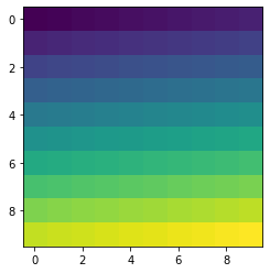
An image can be seen as a 2-dimensional array. To visualise the contents of a numpy array:
[25]:
arr = np.arange(100).reshape(10, 10)

print(arr)

plt.imshow(arr)
[[ 0  1  2  3  4  5  6  7  8  9]
 [10 11 12 13 14 15 16 17 18 19]
 [20 21 22 23 24 25 26 27 28 29]
 [30 31 32 33 34 35 36 37 38 39]
 [40 41 42 43 44 45 46 47 48 49]
 [50 51 52 53 54 55 56 57 58 59]
 [60 61 62 63 64 65 66 67 68 69]
 [70 71 72 73 74 75 76 77 78 79]
 [80 81 82 83 84 85 86 87 88 89]
 [90 91 92 93 94 95 96 97 98 99]]
[25]:
<matplotlib.image.AxesImage at 0x7f1fe1f5b430>
We can use the Pyplot library to load an image using the function imread:
[26]:
im = np.copy(plt.imread("../Supplementary_data/07_Intro_to_numpy/africa.png"))
Let’s display this image using the imshow function.
[27]:
plt.imshow(im)
[27]:
<matplotlib.image.AxesImage at 0x7f1fe1ee4130>
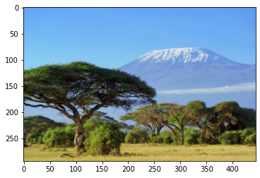
This is a free stock photo of Mount Kilimanjaro, Tanzania. A colour image is normally composed of three layers containing the values of the red, green and blue pixels. When we display an image we see all three colours combined.
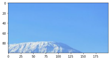
Let’s use the indexing functionality of numpy to select a slice of this image. For example to select the top right corner:
[28]:
plt.imshow(im[:100,-200:,:])
[28]:
<matplotlib.image.AxesImage at 0x7f1fe19fb940>
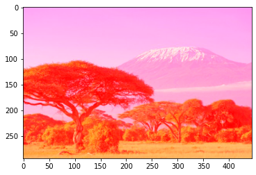
We can also replace values in the ‘red’ layer with the value 255, making the image ‘reddish’. Give it a try:
[29]:
im[:, :, 0] = 255
plt.imshow(im)
Clipping input data to the valid range for imshow with RGB data ([0..1] for floats or [0..255] for integers).
[29]:
<matplotlib.image.AxesImage at 0x7f1fe19dc040>
Recommended next steps
For more advanced information about working with Jupyter Notebooks or JupyterLab, you can explore JupyterLab documentation page.
To continue working through the notebooks in this beginner’s guide, the following notebooks are designed to be worked through in the following order:
Introduction to Numpy (this notebook)
Once you have you have completed the above nine tutorials, join advanced users in exploring:
The “DEA_products” directory in the repository, where you can explore DEA products in depth.
The “How_to_guides” directory, which contains a recipe book of common techniques and methods for analysing DEA data.
The “Real_world_examples” directory, which provides more complex workflows and analysis case studies.
Additional information
License: The code in this notebook is licensed under the Apache License, Version 2.0. Digital Earth Australia data is licensed under the Creative Commons by Attribution 4.0 license.
Contact: If you need assistance, please post a question on the Open Data Cube Discord chat or on the GIS Stack Exchange using the open-data-cube tag (you can view previously asked questions here). If you would like to report an issue with this notebook, you can file one on
GitHub.
Last modified: December 2023
Tags
Browse all available tags on the DEA User Guide’s `Tags Index <>`__
Tags: sandbox compatible, NCI compatible, numpy, matplotlib, plotting, beginner