Parallel processing with Dask 
Compatibility: Notebook currently compatible with both the
NCIandDEA SandboxenvironmentsProducts used: ga_ls8cls9c_gm_cyear_3
Prerequisites: Users of this notebook should have a basic understanding of:
How to run a Jupyter notebook
The basic structure of the DEA satellite datasets
Inspecting available DEA products and measurements
How to load data from DEA
How to plot loaded data
How to run a basic analysis
Background
Dask is a useful tool when working with large analyses (either in space or time) as it breaks data into manageable chunks that can be easily stored in memory. It can also use multiple computing cores to speed up computations. This has numerous benefits for analyses, which will be covered in this notebook.
Description
This notebook covers how to enable Dask as part of loading data, which can allow you to analyse larger areas and longer time-spans without crashing the Digital Earth Australia environments, as well as potentially speeding up your calculations.
Topics covered in this notebook include:
The difference between the standard load command and loading with Dask.
Enabling Dask and the Dask Dashboard.
Setting chunk sizes for data loading.
Loading data with Dask.
Chaining operations together before loading any data and understanding task graphs.
Getting started
To run this introduction to Dask, run all the cells in the notebook starting with the “Load packages” cell. For help with running notebook cells, refer back to the Jupyter Notebooks notebook.
Load packages
The cell below imports the datacube package, which already includes Dask functionality. The sys package provides access to helpful support functions in the dea_tools.dask module, specifically the create_local_dask_cluster function. The dea_tools.plotting module contains the function rgb which will allow us to plot the data we load using Dask.
[1]:
import datacube

import sys
sys.path.insert(1, '../Tools/')
from dea_tools.dask import create_local_dask_cluster
from dea_tools.plotting import rgb
from datacube.utils.masking import mask_invalid_data
Connect to the datacube
The next step is to connect to the datacube database. The resulting dc datacube object can then be used to load data. The app parameter is a unique name used to identify the notebook that does not have any effect on the analysis.
[2]:
dc = datacube.Datacube(app="09_Parallel_processing_with_Dask")
Standard load
By default, the datacube library will not use Dask when loading data. This means that when dc.load() is used, all data relating to the load query will be requested and loaded into memory.
For very large areas or long time spans, this can cause the Jupyter notebook to crash.
For more information on how to use dc.load(), see the Loading data notebook. Below, we show a standard load example:
[3]:
ds = dc.load(product="ga_ls8cls9c_gm_cyear_3",
             measurements=["nbart_red", "nbart_green", "nbart_blue"],
             x=(153.0, 153.8),
             y=(-27.2, -28.0),
             time="2016")
Enabling Dask
One of the major features of Dask is that it can take advantage of multiple CPU cores to speed up computations, which is known as distributed computing. This is good for situations where you need to do a lot of calculations on large datasets.
To set up distributed computing with Dask, you need to first set up a Dask client using the function below:
[4]:
client = create_local_dask_cluster(return_client=True)
Client
Client-bb92ac11-610f-11f0-80d4-a257d99bdb0e
| Connection method: Cluster object | Cluster type: distributed.LocalCluster |
| Dashboard: /user/chad.burton@ga.gov.au/proxy/8787/status |
Cluster Info
LocalCluster
0d136d0c
| Dashboard: /user/chad.burton@ga.gov.au/proxy/8787/status | Workers: 1 |
| Total threads: 2 | Total memory: 15.00 GiB |
| Status: running | Using processes: True |
Scheduler Info
Scheduler
Scheduler-b58c4fad-d723-40eb-806e-e7e3f4a461e7
| Comm: tcp://127.0.0.1:42885 | Workers: 1 |
| Dashboard: /user/chad.burton@ga.gov.au/proxy/8787/status | Total threads: 2 |
| Started: Just now | Total memory: 15.00 GiB |
Workers
Worker: 0
| Comm: tcp://127.0.0.1:42455 | Total threads: 2 |
| Dashboard: /user/chad.burton@ga.gov.au/proxy/41237/status | Memory: 15.00 GiB |
| Nanny: tcp://127.0.0.1:46385 | |
| Local directory: /tmp/dask-scratch-space/worker-trh6qnkd | |
A print out should appear, displaying information about the Client and the Cluster. For now, we’re most interested in the hyperlink after the Dashboard: heading, which should look something like `/user/<username>/proxy/8787/status <>`__, where `<username> <>`__ is your username.
This link provides a way for you to view how any computations you run are progressing. There are two ways to view the dashboard: 1. Click the link, which will open a new tab in your browser 2. Set up the dashboard inside the JupyterLab environment.
We’ll now cover how to do the second option.
Dask dashboard in JupyterLab
On the left-hand menu bar, click the Dask icon, as shown below:

Copy and paste the Dashboard link from the Client print out in the DASK DASHBOARD URL text box:
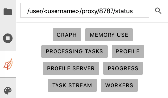
If the url is valid, the buttons should go from grey to orange. Click the orange PROGRESS button on the dask panel, which will open a new tab inside JupyterLab.
To view the Dask window and your active notebook at the same time, drag the new Dask Progress tab to the bottom of the screen.
Now, when you do computations with Dask, you’ll see the progress of the computations in this new Dask window.
Lazy load
When using Dask, the dc.load() function will switch from immediately loading the data to “lazy-loading” the data. This means the data is only loaded when it is going to be used for a calculation, potentially saving time and memory.
Lazy-loading changes the data structure returned from the dc.load() command: the returned xarray.Dataset will be comprised of dask.array objects.
To request lazy-loaded data, add a dask_chunks parameter to your dc.load() call:
[5]:
lazy_ds = dc.load(product="ga_ls8cls9c_gm_cyear_3",
                  measurements=["nbart_red", "nbart_green", "nbart_blue"],
                  x=(153.0, 153.8),
                  y=(-27.2, -28.0),
                  time="2016",
                  dask_chunks={"time": 1, "x": 2048, "y": 2048})

lazy_ds
[5]:
<xarray.Dataset> Size: 62MB
Dimensions:      (time: 1, y: 3384, x: 3064)
Coordinates:
  * time         (time) datetime64[ns] 8B 2016-07-01T23:59:59.999999
  * y            (y) float64 27kB -3.118e+06 -3.118e+06 ... -3.219e+06
  * x            (x) float64 25kB 2.031e+06 2.031e+06 ... 2.123e+06 2.123e+06
    spatial_ref  int32 4B 3577
Data variables:
    nbart_red    (time, y, x) int16 21MB dask.array<chunksize=(1, 2048, 2048), meta=np.ndarray>
    nbart_green  (time, y, x) int16 21MB dask.array<chunksize=(1, 2048, 2048), meta=np.ndarray>
    nbart_blue   (time, y, x) int16 21MB dask.array<chunksize=(1, 2048, 2048), meta=np.ndarray>
Attributes:
    crs:           epsg:3577
grid_mapping: spatial_refThe function should return much faster, as it is not reading any data from disk.
Dask chunks
After adding the dask_chunks parameter to dc.load(), the lazy-loaded data contains dask.array objects with the chunksize listed. The chunksize should match the dask_chunks parameter originally passed to dc.load().
Dask works by breaking up large datasets into chunks, which can be read individually. You may specify the number of pixels in each chunk for each dataset dimension.
For example, we passed the following chunk definition to dc.load():
dask_chunks = {"time": 1, "x": 2048, "y": 2048}
This definition tells Dask to cut the data into chunks containing 2048 pixels in the x and y dimensions and one measurement in the time dimension. For DEA data, we always set "time": 1 in the dask_chunk definition, since the data files only span a single time.
If a chunk size is not provided for a given dimension, or if it set to -1, then the chunk will be set to the size of the array in that dimension. This means all the data in that dimension will be loaded at once, rather than being broken into smaller chunks.
Viewing Dask chunks
To get a visual intuition for how the data has been broken into chunks, we can use the .data attribute provided by xarray. This attribute can be used on individual measurements from the lazy-loaded data. When used in a Jupyter Notebook, it provides a table summarising the size of individual chunks and the number of chunks needed.
An example is shown below, using the nbart_red measurement from the lazy-loaded data:
[6]:
lazy_ds.nbart_red.data
[6]:
|
||||||||||||||||
From the Chunk column of the table, we can see that the data has been broken into four chunks, with each chunk having a shape of (1 time, 2048 pixels, 2048 pixels) and taking up a maximum of 8.00MiB of memory. Comparing this with the Array column, using Dask means that we can load four lots of less than 8.00MiB, rather than one lot of 19.77MiB.
This is valuable when it comes to working with large areas or time-spans, as the entire array may not always fit into the memory available. Breaking large datasets into chunks and loading chunks one at a time means that you can do computations over large areas without crashing the DEA environment.
Loading lazy data
When working with lazy-loaded data, you have to specifically ask Dask to read and load data when you want to use it. Until you do this, the lazy-loaded dataset only knows where the data is, not its values.
To load the data from disk, call .load() on the DataArray or Dataset. If you opened the Dask progress window, you should see the computation proceed there.
[7]:
loaded_ds = lazy_ds.load()
loaded_ds
[7]:
<xarray.Dataset> Size: 62MB
Dimensions:      (time: 1, y: 3384, x: 3064)
Coordinates:
  * time         (time) datetime64[ns] 8B 2016-07-01T23:59:59.999999
  * y            (y) float64 27kB -3.118e+06 -3.118e+06 ... -3.219e+06
  * x            (x) float64 25kB 2.031e+06 2.031e+06 ... 2.123e+06 2.123e+06
    spatial_ref  int32 4B 3577
Data variables:
    nbart_red    (time, y, x) int16 21MB 712 654 595 580 554 ... 106 106 109 105
    nbart_green  (time, y, x) int16 21MB 677 606 551 524 509 ... 161 163 167 163
    nbart_blue   (time, y, x) int16 21MB 382 341 322 313 308 ... 325 325 324 323
Attributes:
    crs:           epsg:3577
grid_mapping: spatial_refThe Dask arrays constructed by the lazy load, e.g.:
red (time, y, x) uint16 dask.array<chunksize=(1, 2048, 2048), meta=np.ndarray>
have now been replaced with actual numbers:
red (time, y, x) uint16 10967 11105 10773 10660 ... 12431 12410 12313
After applying the .load() command, the lazy-loaded data is the same as the data loaded from the first query.
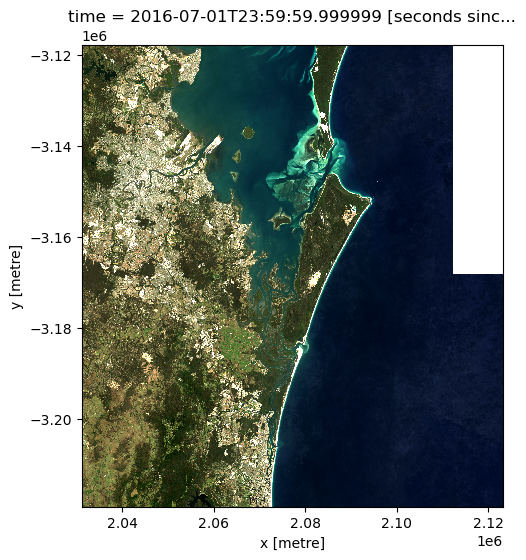
We can now plot the data to verify it loaded correctly:
[8]:
# Set invalid nodata pixels to NaN
loaded_ds_cleaned = mask_invalid_data(loaded_ds)
[9]:
rgb(loaded_ds_cleaned, bands=["nbart_red", "nbart_green", "nbart_blue"])
Lazy operations
In addition to breaking data into smaller chunks that fit in memory, Dask has another advantage in that it can track how you want to work with the data, then only perform the necessary operations later.
We’ll now explore how to do this by calculating the normalised difference vegetation index (NDVI) for our data. To do this, we’ll perform the lazy-load operation again, this time adding the near-infrared band (nir) to the dc.load() command:
[10]:
lazy_ds = dc.load(product="ga_ls8cls9c_gm_cyear_3",
                  measurements=["nbart_red", "nbart_green", "nbart_blue", "nbart_nir"],
                  x=(153.0, 153.8),
                  y=(-27.2, -28.0),
                  time="2016",
                  dask_chunks={"time": 1, "x": 2048, "y": 2048})

lazy_ds
[10]:
<xarray.Dataset> Size: 83MB
Dimensions:      (time: 1, y: 3384, x: 3064)
Coordinates:
  * time         (time) datetime64[ns] 8B 2016-07-01T23:59:59.999999
  * y            (y) float64 27kB -3.118e+06 -3.118e+06 ... -3.219e+06
  * x            (x) float64 25kB 2.031e+06 2.031e+06 ... 2.123e+06 2.123e+06
    spatial_ref  int32 4B 3577
Data variables:
    nbart_red    (time, y, x) int16 21MB dask.array<chunksize=(1, 2048, 2048), meta=np.ndarray>
    nbart_green  (time, y, x) int16 21MB dask.array<chunksize=(1, 2048, 2048), meta=np.ndarray>
    nbart_blue   (time, y, x) int16 21MB dask.array<chunksize=(1, 2048, 2048), meta=np.ndarray>
    nbart_nir    (time, y, x) int16 21MB dask.array<chunksize=(1, 2048, 2048), meta=np.ndarray>
Attributes:
    crs:           epsg:3577
grid_mapping: spatial_refTask graphs
When using lazy-loading, Dask breaks up the loading operation into a series of steps. A useful way to visualise the steps is the task graph, which can be accessed by adding the .visualize() method to a .data call:
[11]:
lazy_ds.nbart_red.data.visualize()
[11]:
The task graph is read from bottom to top.
The rectangles at the bottom of the graph are the database entries describing the files that need to be read to load the data.
Above the rectangles are individual load commands that will do the reading. There is one for each chunk. The arrows describe which files need to be read for each operation: the chunk on the left needs data from all four database entries (i.e. four arrows), whereas the chunk on the right only needs data from one.
At the very top are the indexes of the chunks that will make up the final array.
Adding more tasks
The power of this method comes from chaining tasks together before loading the data. This is because Dask will only load the data that is required by the final operation in the chain.
We can demonstrate this by requesting only a small portion of the red band. If we do this for the lazy-loaded data, we can view the new task graph:
[12]:
extract_from_red = lazy_ds.nbart_red[:, 100:200, 100:200]
extract_from_red.data.visualize()
[12]:
Notice that the new task getitem has been added, and that it only applies to the left-most chunk. If we call .load() on the extract_from_red Dask array, Dask trace the operation back through the graph to find only the relevant data. This can save both memory and time.
We can establish that the above operation yields the same result as loading the data without Dask and subsetting it by running the command below:
[13]:
lazy_red_subset = extract_from_red.load()
data_red_subset = ds.nbart_red[:, 100:200, 100:200]

print(f"The loaded arrays match: {lazy_red_subset.equals(data_red_subset)}")
The loaded arrays match: True
Since the arrays are the same, it is worth using lazy-loading to chain operations together, then calling .load() only when you’re ready to get the answer. This saves time and memory, since Dask will only load the input data that is required to get the final output. In this example, the lazy-load only needed to load a small section of the nbart_red band, whereas the original load to get data had to load the nbart_red, nbart_green and nbart_blue bands, then subset the
nbart_red band, meaning time was spent loading data that wasn’t used.
Multiple tasks
The power of using lazy-loading in Dask is that you can continue to chain operations together until you are ready to get the answer.
Here, we chain multiple steps together to calculate a new band for our array. Specifically, we use the nbart_red and nbart_nir bands to calculate the Normalised Difference Vegetation Index (NDVI), which can help identify areas of healthy vegetation. For remote sensing data such as satellite imagery, it is defined as:
where \(\text{NIR}\) is the near-infrared band of the data, and \(\text{Red}\) is the red band:
[14]:
band_diff = lazy_ds.nbart_nir - lazy_ds.nbart_red
band_sum = lazy_ds.nbart_nir + lazy_ds.nbart_red

lazy_ds["ndvi"] = band_diff / band_sum
Doing this adds the new ndvi Dask array to the lazy_data dataset:
[15]:
lazy_ds
[15]:
<xarray.Dataset> Size: 166MB
Dimensions:      (time: 1, y: 3384, x: 3064)
Coordinates:
  * time         (time) datetime64[ns] 8B 2016-07-01T23:59:59.999999
  * y            (y) float64 27kB -3.118e+06 -3.118e+06 ... -3.219e+06
  * x            (x) float64 25kB 2.031e+06 2.031e+06 ... 2.123e+06 2.123e+06
    spatial_ref  int32 4B 3577
Data variables:
    nbart_red    (time, y, x) int16 21MB dask.array<chunksize=(1, 2048, 2048), meta=np.ndarray>
    nbart_green  (time, y, x) int16 21MB dask.array<chunksize=(1, 2048, 2048), meta=np.ndarray>
    nbart_blue   (time, y, x) int16 21MB dask.array<chunksize=(1, 2048, 2048), meta=np.ndarray>
    nbart_nir    (time, y, x) int16 21MB dask.array<chunksize=(1, 2048, 2048), meta=np.ndarray>
    ndvi         (time, y, x) float64 83MB dask.array<chunksize=(1, 2048, 2048), meta=np.ndarray>
Attributes:
    crs:           epsg:3577
grid_mapping: spatial_refNow that the operation is defined, we can view its task graph:
[16]:
lazy_ds.ndvi.data.visualize()
[16]:
Reading the graph bottom-to-top, we can see the equation taking place. The add and sub are performed on each band before being divided (truediv).
We can see how each output chunk is independent from the others. This means we could calculate each chunk without ever having to load all of the bands into memory at the same time.
Finally, we can calculate the NDVI values and load the result into memory by calling the .load() command. We’ll store the result in the ndvi_load variable:
[17]:
ndvi_load = lazy_ds.ndvi.load()
ndvi_load
[17]:
<xarray.DataArray 'ndvi' (time: 1, y: 3384, x: 3064)> Size: 83MB
array([[[ 0.57631657,  0.59022556,  0.61237785, ..., -0.        ,
         -0.        , -0.        ],
        [ 0.58010375,  0.60680908,  0.5964493 , ..., -0.        ,
         -0.        , -0.        ],
        [ 0.55622289,  0.59569458,  0.57683598, ..., -0.        ,
         -0.        , -0.        ],
        ...,
        [ 0.67173027,  0.67957746,  0.66293393, ..., -0.12903226,
         -0.10880829, -0.1147541 ],
        [ 0.610957  ,  0.6123348 ,  0.6242236 , ..., -0.12299465,
         -0.11458333, -0.125     ],
        [ 0.57268425,  0.57101072,  0.57369897, ..., -0.10994764,
         -0.1010101 , -0.10526316]]])
Coordinates:
  * time         (time) datetime64[ns] 8B 2016-07-01T23:59:59.999999
  * y            (y) float64 27kB -3.118e+06 -3.118e+06 ... -3.219e+06
  * x            (x) float64 25kB 2.031e+06 2.031e+06 ... 2.123e+06 2.123e+06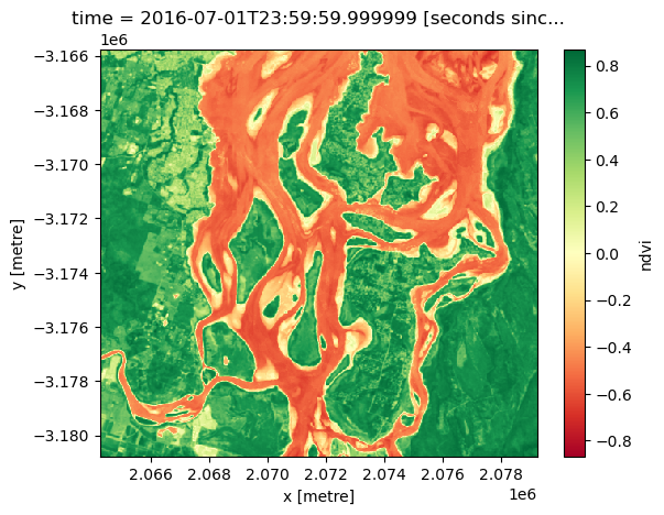
spatial_ref int32 4B 3577We can plot a subset of our NDVI data to verify that Dask correctly calculated our sequence of tasks. Vegetation should appear in green (indicating high NDVI values), and non-vegetation in red (indicating low NDVI values, e.g. over water):
[18]:
ndvi_load[:, 1600:2100, 1100:1600].plot(cmap="RdYlGn")
[18]:
<matplotlib.collections.QuadMesh at 0x7fc47a9bdd80>
Note that running the .load() command also modifies the ndvi entry in the lazy_load dataset:
[19]:
lazy_ds
[19]:
<xarray.Dataset> Size: 166MB
Dimensions: (time: 1, y: 3384, x: 3064)
Coordinates:
* time (time) datetime64[ns] 8B 2016-07-01T23:59:59.999999
* y (y) float64 27kB -3.118e+06 -3.118e+06 ... -3.219e+06
* x (x) float64 25kB 2.031e+06 2.031e+06 ... 2.123e+06 2.123e+06
spatial_ref int32 4B 3577
Data variables:
nbart_red (time, y, x) int16 21MB dask.array<chunksize=(1, 2048, 2048), meta=np.ndarray>
nbart_green (time, y, x) int16 21MB dask.array<chunksize=(1, 2048, 2048), meta=np.ndarray>
nbart_blue (time, y, x) int16 21MB dask.array<chunksize=(1, 2048, 2048), meta=np.ndarray>
nbart_nir (time, y, x) int16 21MB dask.array<chunksize=(1, 2048, 2048), meta=np.ndarray>
ndvi (time, y, x) float64 83MB 0.5763 0.5902 ... -0.101 -0.1053
Attributes:
crs: epsg:3577
grid_mapping: spatial_refYou can see that ndvi is a number, whereas all the other variables are Dask arrays.
Keeping variables as Dask arrays
If you wanted to calculate the NDVI values, but leave ndvi as a dask array in lazy_load, you can use the .compute() command instead.
To demonstrate this, we first redefine the ndvi variable so that it becomes a Dask array again:
[20]:
lazy_ds["ndvi"] = band_diff / band_sum
lazy_ds
[20]:
<xarray.Dataset> Size: 166MB
Dimensions: (time: 1, y: 3384, x: 3064)
Coordinates:
* time (time) datetime64[ns] 8B 2016-07-01T23:59:59.999999
* y (y) float64 27kB -3.118e+06 -3.118e+06 ... -3.219e+06
* x (x) float64 25kB 2.031e+06 2.031e+06 ... 2.123e+06 2.123e+06
spatial_ref int32 4B 3577
Data variables:
nbart_red (time, y, x) int16 21MB dask.array<chunksize=(1, 2048, 2048), meta=np.ndarray>
nbart_green (time, y, x) int16 21MB dask.array<chunksize=(1, 2048, 2048), meta=np.ndarray>
nbart_blue (time, y, x) int16 21MB dask.array<chunksize=(1, 2048, 2048), meta=np.ndarray>
nbart_nir (time, y, x) int16 21MB dask.array<chunksize=(1, 2048, 2048), meta=np.ndarray>
ndvi (time, y, x) float64 83MB dask.array<chunksize=(1, 2048, 2048), meta=np.ndarray>
Attributes:
crs: epsg:3577
grid_mapping: spatial_refNow, we perform the same steps as before to calculate NDVI, but use .compute() instead of .load():
[21]:
ndvi_compute = lazy_ds.ndvi.compute()
ndvi_compute
[21]:
<xarray.DataArray 'ndvi' (time: 1, y: 3384, x: 3064)> Size: 83MB
array([[[ 0.57631657,  0.59022556,  0.61237785, ..., -0.        ,
         -0.        , -0.        ],
        [ 0.58010375,  0.60680908,  0.5964493 , ..., -0.        ,
         -0.        , -0.        ],
        [ 0.55622289,  0.59569458,  0.57683598, ..., -0.        ,
         -0.        , -0.        ],
        ...,
        [ 0.67173027,  0.67957746,  0.66293393, ..., -0.12903226,
         -0.10880829, -0.1147541 ],
        [ 0.610957  ,  0.6123348 ,  0.6242236 , ..., -0.12299465,
         -0.11458333, -0.125     ],
        [ 0.57268425,  0.57101072,  0.57369897, ..., -0.10994764,
         -0.1010101 , -0.10526316]]])
Coordinates:
* time (time) datetime64[ns] 8B 2016-07-01T23:59:59.999999
* y (y) float64 27kB -3.118e+06 -3.118e+06 ... -3.219e+06
* x (x) float64 25kB 2.031e+06 2.031e+06 ... 2.123e+06 2.123e+06
spatial_ref int32 4B 3577You can see that the values have been calculated, but as shown below, the ndvi variable is kept as a Dask array.
[22]:
lazy_ds
[22]:
<xarray.Dataset> Size: 166MB
Dimensions:      (time: 1, y: 3384, x: 3064)
Coordinates:
  * time         (time) datetime64[ns] 8B 2016-07-01T23:59:59.999999
  * y            (y) float64 27kB -3.118e+06 -3.118e+06 ... -3.219e+06
  * x            (x) float64 25kB 2.031e+06 2.031e+06 ... 2.123e+06 2.123e+06
    spatial_ref  int32 4B 3577
Data variables:
    nbart_red    (time, y, x) int16 21MB dask.array<chunksize=(1, 2048, 2048), meta=np.ndarray>
    nbart_green  (time, y, x) int16 21MB dask.array<chunksize=(1, 2048, 2048), meta=np.ndarray>
    nbart_blue   (time, y, x) int16 21MB dask.array<chunksize=(1, 2048, 2048), meta=np.ndarray>
    nbart_nir    (time, y, x) int16 21MB dask.array<chunksize=(1, 2048, 2048), meta=np.ndarray>
    ndvi         (time, y, x) float64 83MB dask.array<chunksize=(1, 2048, 2048), meta=np.ndarray>
Attributes:
    crs:           epsg:3577
grid_mapping: spatial_refUsing .compute() can allow you to calculate in-between steps and store the results, without modifying the original Dask dataset or array. However, be careful when using .compute(), as it may lead to confusion about what you have and have not modified, as well as multiple computations of the same quantity.
Shutting down the Dask client
To free up computing resources for future work, we can close the Dask client once we are finished:
[23]:
client.close()
Recommended next steps
Further resources
For further reading on how Dask works, and how it is used by xarray, see these resources:
Other notebooks
You have now completed the full beginner’s guide tutorial!
Parallel processing with Dask (this notebook)
You can now join more advanced users in exploring:
The “DEA_products” directory in the repository, where you can explore DEA products in depth.
The “How_to_guides” directory, which contains a recipe book of common techniques and methods for analysing DEA data.
The “Real_world_examples” directory, which provides more complex workflows and analysis case studies.
Additional information
License: The code in this notebook is licensed under the Apache License, Version 2.0. Digital Earth Australia data is licensed under the Creative Commons by Attribution 4.0 license.
Contact: If you need assistance, please post a question on the Open Data Cube Discord chat or on the GIS Stack Exchange using the open-data-cube tag (you can view previously asked questions here). If you would like to report an issue with this notebook, you can file one on
GitHub.
Last modified: June 2024
Compatible ``datacube`` version:
[24]:
print(datacube.__version__)
1.8.19
Tags
Tags: sandbox compatible, NCI compatible, landsat 8, annual geomedian, NDVI, plotting, dea_plotting, rgb, Dask, parallel processing, lazy loading, beginner
[ ]: