Handling Cloud-Optimised Geotiff overviews

• Sign up to the DEA Sandbox to run this notebook interactively from a browser

• Compatibility: Notebook currently compatible with the DEA Sandbox environment

• Products used:

  • ga_ls_landcover_class_cyear_3;

  • Landcover continental COG mosaics

• Prerequisites: It is recommended to first read the notebook COG_mosaics

Background

Some DEA products are provided as continental-scale mosaics in the form of Cloud Optimised GeoTIFFs (COGs). These mosaics enable the streaming of DEA data via GIS software and are accompanied by Virtual Raster (VRT) files, which are lightweight wrappers that automatically provide visualisation styling when streaming the data.

COGs include overviews (or pyramids) that approximate the raw data array at a coarser spatial resolution by applying a resampling algorithm such as NEAREST, BILINEAR, or MODE. This allows data to be streamed at a continental scale much faster than if the entire array were to be loaded at native resolution.

While the main advantage of COGs lies in their use within GIS software, they can also be accessed programmatically using languages such as Python, with packages like rioxarray or gdal.

Although using the native resolution of the data array is recommended, it is also possible to access the coarser overviews to reduce computational demand when working on smaller machines, or when the data resolution needs to match that of another, coarser resolution product.

Description

This notebook explores how to perform the following actions: * Access a mosaic Cloud-Optimised GeoTIFFs (COGs) from the DEA S3 repository * Load the data for our ROI using different overviews and observe the differences in Land Cover classes’ extent

---

Getting started

Load packages

Import the Python packages needed for this notebook.

import sys
import rioxarray
import numpy as np
from osgeo import gdal
from odc.geo.xr import crop
import matplotlib.pyplot as plt
from odc.geo import BoundingBox

sys.path.insert(1, "../Tools/")
from dea_tools.plotting import display_map
from dea_tools.landcover import lc_colourmap, get_colour_scheme, make_colourbar

Analysis Parameters

In this notebook, we will use DEA Land Cover Level 3 as an example, and the analysis parameters below reflect this. You can see which other products are distributed as mosaics here: Continental Cloud-Optimised GeoTIFF Mosaics.

• lat, lon: The central latitude and longitude to analyse. In this example we’ll define a region around Canberra, ACT.

• buffer: The number of square degrees to load around the central latitude and longitude.

• product: The name of the DEA products to load, in the example we will use DEA Landcover

• version: The latest version of DEA Landcover is '2-0-0'

• level: DEA Landcover has a two measurements, 'level3' and 'level4'

• year: The year of interest to load. DEA Landcover is an annual product starting in 1988

# Coordinates for Canberra region
lat, lon = -35.325, 149.0918
buffer = 0.5

# Define variables needed to obtain the DEA Land Cover Level 3 data.
# Currently, the most recent version is 2-0-0.
product = 'ga_ls_landcover_class_cyear_3'
version = '2-0-0'
level = 'level3'

# Set year of interest
year = 2024

View your study area

In the default example the bounding box covers the region around Canberra.

bbox = BoundingBox(
    left= lon - buffer,
    bottom=lat - buffer,
    right=lon + buffer,
    top=lat + buffer,
    crs="EPSG:4326"
)

bbox.explore()

Make this Notebook Trusted to load map: File -> Trust Notebook

Load data from the continental mosaic and crop it to the ROI

We will read the COG continental mosaic from the DEA S3 repository and see how many overviews are included in the file.

# URL to DEA continental mosaics
cog_url = f'https://data.dea.ga.gov.au/derivative/{product}/{version}/continental_mosaics/{year}--P1Y/{product}_mosaic_{year}--P1Y_{level}.tif'

# We will use gdal to quickly gather information on the overviews contained in the COG
# let's add the vsicurl driver to facilitate reading the file with GDAL
cog = gdal.Open(f'/vsicurl/{cog_url}', gdal.GA_ReadOnly)

# We select the first and only band in the mosaic
band = cog.GetRasterBand(1)
overview_count = band.GetOverviewCount()

# Get base image geotransform
gt = cog.GetGeoTransform()
base_res_x = abs(gt[1])
base_res_y = abs(gt[5])
base_xsize = band.XSize
base_ysize = band.YSize

print(f"Native COG resolution: {base_res_x:.0f}, {base_res_y:.0f}")
print(f"Native COG size: {base_xsize} x {base_ysize} pixels\n")

for i in range(overview_count):
    ov = band.GetOverview(i)
    scale_x = base_xsize / ov.XSize
    scale_y = base_ysize / ov.YSize
    ov_res_x = base_res_x * scale_x
    ov_res_y = base_res_y * scale_y
    print(
        f"Overview {i}: size = {ov.XSize} x {ov.YSize} pixels, "
        f"resolution = ({ov_res_x:.0f}, {ov_res_y:.0f})"
    )

Native COG resolution: 30, 30
Native COG size: 137600 x 128000 pixels

Overview 0: size = 68800 x 64000 pixels, resolution = (60, 60)
Overview 1: size = 34400 x 32000 pixels, resolution = (120, 120)
Overview 2: size = 17200 x 16000 pixels, resolution = (240, 240)
Overview 3: size = 8600 x 8000 pixels, resolution = (480, 480)
Overview 4: size = 4300 x 4000 pixels, resolution = (960, 960)
Overview 5: size = 2150 x 2000 pixels, resolution = (1920, 1920)
Overview 6: size = 1075 x 1000 pixels, resolution = (3840, 3840)

/env/lib/python3.10/site-packages/osgeo/gdal.py:311: FutureWarning: Neither gdal.UseExceptions() nor gdal.DontUseExceptions() has been explicitly called. In GDAL 4.0, exceptions will be enabled by default.
  warnings.warn(

We observed that there are seven overviews, each halving the size of the array at every level. We will load the data at a medium overview level (overview_level = 2) using the argument overview_level in rioxarray.open_rasterio().

For categorical data such as DEA Land Cover, the overviews were generated using the mode algorithm. This means that pixels at the native resolution representing uncommon or sparsely distributed classes might be lost during resampling.

# Define the overview level of interest
overview_level = 2

# Read a specific overview of the COG with rioxarray and check what the CRS of the file is
cog_array = rioxarray.open_rasterio(cog_url, overview_level=overview_level)
cog_crs = cog_array.rio.crs
print(f'The CRS of the COG is {cog_crs}')

The CRS of the COG is EPSG:3577

Now we can crop the array to our ROI.

roi_geom = bbox.boundary().convex_hull

cog_roi = crop(cog_array, roi_geom)
print(f'The CRS of the cropped COG is {cog_roi.rio.crs}')
print(f'The shape of the array is {cog_roi.shape}')

The CRS of the cropped COG is EPSG:3577
The shape of the array is (1, 510, 437)

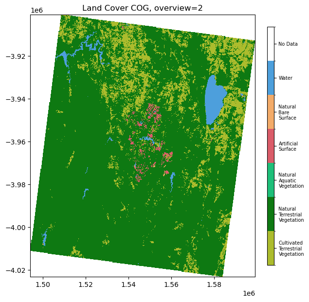
Let’s quickly visualise the extent of the final array.

fig, ax = plt.subplots(1, 1, figsize=(7, 7), sharey=True)

# Set up the colormap
colour_scheme = get_colour_scheme(level)
cmap, norm = lc_colourmap(colour_scheme)
im = cog_roi.plot(cmap=cmap, norm=norm, ax=ax, add_labels=False, add_colorbar=False)
ax.set_title(f"Land Cover COG, overview={overview_level}", fontsize=12)
make_colourbar(fig, ax, measurement=level, labelsize=7, horizontal=False);

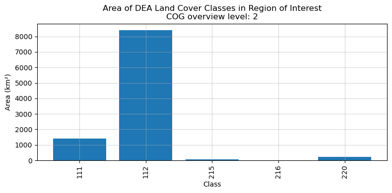
Analyse the data

Now we can include the data in any workflow that involves data arrays. Here we will perform a simple value count as an example and observe the extent of each land cover class in our bounding box

You can see the name corresponding to each class value in the DEA Knowledge Hub.

# First we convert our array to a 1D vector and mask out NaN values
data_1d = cog_roi.values.flatten()
data_1d = data_1d[~np.isnan(data_1d)]

# Let's count the number of pixels in each class
classes, counts = np.unique(data_1d, return_counts=True)

# Define the pixel size of the selected overview
pixel_size_m = cog_array.odc.geobox.resolution.x

# Calculate the area of one pixel
pixel_area_km2 = (pixel_size_m ** 2) / 1e6

# Calculate the total area of each class
area_km2 = counts * pixel_area_km2

We will visualise the areal extent of the Land Cover classes with a bar chart.

x_pos = np.arange(len(classes)) # positions of x axis ticks

plt.figure(figsize=(8,4))

# Plot area in km² per class
plt.bar(x_pos, area_km2)

plt.xlabel('Class')
plt.ylabel('Area (km²)')
plt.title(f'Area of DEA Land Cover Classes in Region of Interest\nCOG overview level: {overview_level}')

plt.xticks(x_pos, [int(c) for c in classes], rotation=90)
plt.grid(alpha=0.5)
plt.tight_layout();

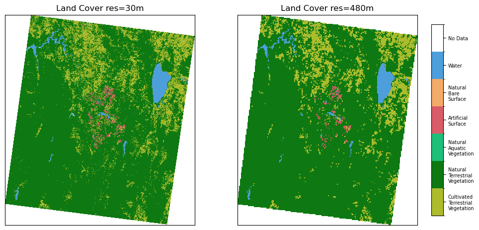
Compare different overviews

In this final section, we will quickly explore the differences between overviews to raise awareness on the caveats associated with using a resampled product, particularly when representing categorical data.

Load two different levels

Note, To load the native resolution, we need to remove the overview_level parameter

# Get the data in the native resolution (30 m) and crop it to our ROI
fine_cog = rioxarray.open_rasterio(cog_url)
fine_cog = crop(fine_cog, roi_geom)

# Repeat for a higher overview
coarse_overview_level = 3
coarse_cog = rioxarray.open_rasterio(cog_url, overview_level=coarse_overview_level)
coarse_cog= crop(coarse_cog, roi_geom)

Plot side by side

We can observe how resampling to a much coarser resolution has changed the pixel values and the look of the landscape.

fig, ax = plt.subplots(1, 2, figsize=(12, 5.5), sharey=True)

# Set up the colour map
colour_scheme = get_colour_scheme(level)
cmap, norm = lc_colourmap(colour_scheme)
im = fine_cog.plot(cmap=cmap, norm=norm, ax=ax[0], add_labels=False, add_colorbar=False)
ax[0].set_title(f"Land Cover res={int(fine_cog.odc.geobox.resolution.x)}m", fontsize=12);

im = coarse_cog.plot(cmap=cmap, norm=norm, ax=ax[1], add_labels=False, add_colorbar=False)
ax[1].set_title(f"Land Cover res={int(coarse_cog.odc.geobox.resolution.x)}m", fontsize=12);
make_colourbar(fig, ax[1], measurement=level, labelsize=7, horizontal=False)

for a in ax.ravel():
    a.axes.get_xaxis().set_ticks([])
    a.axes.get_yaxis().set_ticks([]);

Find the area of each class

# Finest overview (30 m spatial resolution)
fine_data_1d = fine_cog.values.flatten()
fine_data_1d = fine_data_1d[~np.isnan(fine_data_1d)]

fine_classes, fine_counts = np.unique(fine_data_1d, return_counts=True)

fine_pixel_size = fine_cog.odc.geobox.resolution.x # effectively this is 30 m for the overview level 0
fine_pixel_area_km2 = (fine_pixel_size ** 2) / 1e6

# Coarsest overview
coarse_data_1d = coarse_cog.values.flatten()
coarse_data_1d = coarse_data_1d[~np.isnan(coarse_data_1d)]

coarse_classes, coarse_counts = np.unique(coarse_data_1d, return_counts=True)

coarse_pixel_size = coarse_cog.odc.geobox.resolution.x
coarse_pixel_area_km2 = (coarse_pixel_size ** 2) / 1e6

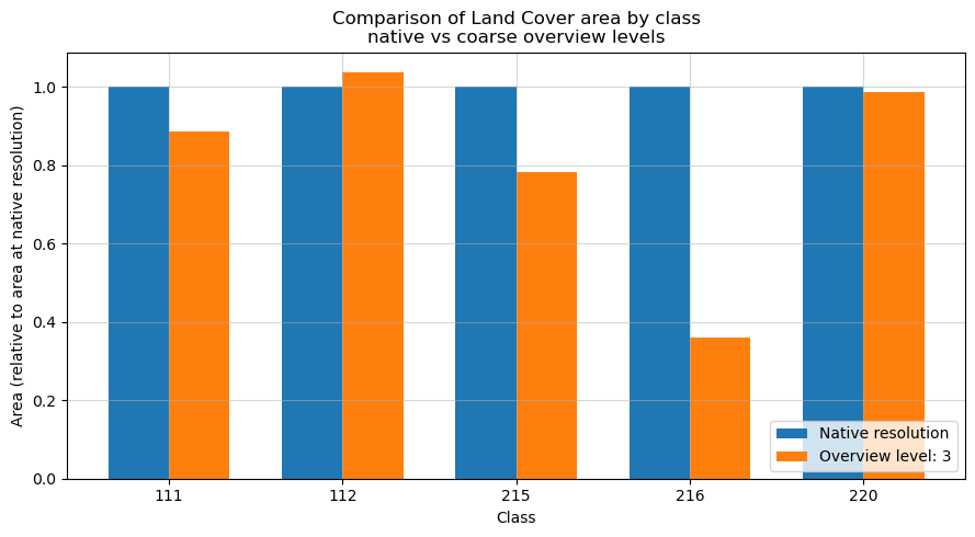
Plot the difference in class areas

Finally, by plotting the class extents of the two overviews side by side, we observe that the extent of some less common classes decreases at the coarser resolution, while the area of other more widespread classes increases.

Class area is expressed as relative to the total class area in the fine resolution overiew (i.e. the 30m resolution dataset). This means all the values for the Native resolution columns will be 1, while the coarse overviews will be either greater or lesser than 1 depending on how the area has changed following the resampling.

It’s important to note that a high relative change does not necessarily correspond to a substantial shift in absolute extent. Rare or sparsely distributed classes with very small absolute areas can show large relative changes at coarser overviews, even though their overall contribution to the landscape remains minimal.

# Combine unique classes from fine and coarse overviews into a single sorted array
# Remove no-data counts
all_classes = np.union1d(fine_classes, coarse_classes)[0:-1]

# Create dictionaries to store counts by class
fine_dict = dict(zip(fine_classes, fine_counts))
coarse_dict = dict(zip(coarse_classes, coarse_counts))

# Align counts to all_classes. Use 0 if class not in one overview
fine_aligned_counts = np.array([fine_dict.get(c, 0) for c in all_classes])
coarse_aligned_counts = np.array([coarse_dict.get(c, 0) for c in all_classes])

# Convert counts to area (km2)
fine_aligned_area_km2 = fine_aligned_counts * fine_pixel_area_km2
coarse_aligned_area_km2 = coarse_aligned_counts * coarse_pixel_area_km2

# Normalise area to the fine resolution. This allows to visualise the relative change of the classes' extent
coarse_aligned_area_km2 = coarse_aligned_area_km2/fine_aligned_area_km2
fine_aligned_area_km2 = fine_aligned_area_km2/fine_aligned_area_km2

x_pos = np.arange(len(all_classes))
width = 0.35

# Plot bars side-by-side comparing fine and coarse overview areas
plt.figure(figsize=(9, 5))
plt.bar(
    x_pos - width / 2,  # -width/2 shifts bars to the left
    fine_aligned_area_km2,
    width,
    label=f"Native resolution",
)

plt.bar(
    x_pos + width / 2,
    coarse_aligned_area_km2,
    width,
    label=f"Overview level: {coarse_overview_level}",
)

plt.xlabel("Class")
plt.ylabel("Area (relative to area at native resolution)")
plt.title("Comparison of Land Cover area by class\nnative vs coarse overview levels")
plt.xticks(x_pos, [int(c) for c in all_classes])
plt.legend(loc='lower right')
plt.grid(alpha=0.5)
plt.tight_layout();

---

Additional information

License: The code in this notebook is licensed under the Apache License, Version 2.0. Digital Earth Australia data is licensed under the Creative Commons by Attribution 4.0 license.

Contact: If you need assistance, please post a question on the Open Data Cube Discord chat or on the GIS Stack Exchange using the open-data-cube tag (you can view previously asked questions here). If you would like to report an issue with this notebook, you can file one on GitHub.

Last modified: October 2025

Tags

**Tags**: :index:`sandbox compatible`, :index:`Landsat`, :index:`COG`, :index:`mosaic`, :index:`continental`, :index:`overviews`, :index:`pyramids`