Accessing Gridded Climate Data 
Sign up to the DEA Sandbox to run this notebook interactively from a browser
Compatibility: Notebook currently compatible with the
DEA Sandbox&NCIenvironmentsProducts used: ERA5 and ANUClim (these datasets are external to the Digital Earth Australia platform)
Background & Description
This notebook demonstrates how to access and use Australian-specific climate data stored on the National Computing Infrastructure (NCI), and global climate reanalysis data (ERA5) hosted on Google’s cloud infrastructure. The content is structured into two parts.
The first section shows how to access an Australian climate dataset through the THREDDS platform. NCI’s THREDDS provides a wide range of climate, satellite, and other gridded environmental datasets, which can be accessed programmatically via
xarray.The second section focuses on the use of a pre-processed version of the ECMWF Reanalysis v5 (ERA5) Climate Fields. These datasets are also accessed using
xarray.
Note: Additional details about the datasets are provided further in the notebook.
Load packages
Import Python packages that are used for the analysis.
[1]:
%matplotlib inline

import os
import gcsfs
import requests
import datacube
import xarray as xr
import pandas as pd
import numpy as np
import contextily as ctx
import geopandas as gpd
from bs4 import BeautifulSoup
import matplotlib.pyplot as plt
from odc.geo.xr import assign_crs
from odc.geo.geom import Geometry, BoundingBox

import sys
sys.path.insert(1, '../Tools/')
from dea_tools.dask import create_local_dask_cluster
Analysis parameters
The following code cell is used to define variable needed later.
vector_path: a file path to the polygon that defines our analysis region, the default example uses a boundary of Victoria.
[2]:
# Boundary of victoria
vector_path = '../Supplementary_data/External_data_Climate/victoria_boundary.geojson'
Section 1: ANUClim climate data
In the first section of this notebook, we demonstrates retrieval of the Australian National University’s Climate data product (‘ANUClim’). These datasets are produced using topographically conditional spatial interpolation of Australia’s extensive network of weather stations.
The available variables include: * tavg: Average surface air temperature * rain: Total precipitation * vpd : Vapour pressure deficit * srad: Incoming solar radiation * evap: Pan evaporation
The entire archive can be viewed here
Data is available at a daily and monthly cadence, and has a 1 x 1 km spatial resolution, making it one of the highest resolution climate data products available for Australia. The time range of the data depends on the climate variable. For example, rainfall goes back to 1900, while air temperature begins in 1960. Data is updated annually.
Note: ANUClim is stored in the
'EPSG:4283'projection
Analysis parameters for ANUClim
var: the climate variable to load.cadence: specifies whether to load monthly or daily data. Must be either ‘month’ or ‘day’.year_start&year_end: the year range of data you want to load, use integer values here.
[3]:
# Which variable should we load?
var = 'rain' # other options: vpd, srad, rain, evap,  tavg

# Define the cadence of the data to load
cadence= 'month' # other options: day

# Define the time window (inclusive of end year) (use integers only)
year_start, year_end = 2020, 2020
Load our region of interest
[4]:
# open the vector file
gdf = gpd.read_file(vector_path)

# convert to GDA94 to match ANUClim's CRS
gdf = gdf.to_crs('epsg:4283')

# define bounding box of the geometry
# we'll use this to select data before masking
bb = gdf.total_bounds
Load the climate data through THREDDS
Extract the links for loading the target year data from THREDDS using xarray.
[5]:
# the top level folder on the NCI
thredds_data_link = 'https://thredds.nci.org.au/thredds/dodsC/gh70/ANUClimate/v2-0/stable/'
thredds_catalog_link=f'https://thredds.nci.org.au/thredds/catalog/gh70/ANUClimate/v2-0/stable/{cadence}/'

# list of years to load
years = [str(i) for i in range(year_start, year_end+1)]

i=0
pp = []

# loop through years and load
for y in years:
    print(" {:02}/{:02}\r".format(i + 1, len(years)), end="")

    # get list of all the file links on the THREDDS server
    ff = f'{thredds_catalog_link}{var}/{y}/catalog.html'
    soup = BeautifulSoup(requests.get(ff).content, "html.parser")

    # extract just the href links
    file_names = []
    for link in soup.select('a[href*=".html"]'): # loop over all <a> elements where the href attribute contains ".html"
        href = link["href"]
        if "dataset" in href: # add only file names of datasets to list
            file_names.append(href)

    # create a list of links for xarray
    list_of_links = [thredds_data_link+f.replace('catalog.html?dataset=gh70/', '') for f in file_names]

    # open with xarray and tidy up
    ds = xr.open_mfdataset(list_of_links)
    ds = assign_crs(ds, crs='epsg:4283') #GDA94
    ds = ds.drop_vars('crs')[var]
    ds.attrs['nodata'] = np.nan

    # select data from within the bounding box of the geometry
    # this is faster than masking, which we can do later
    ds = ds.sel(lat=slice(bb[3], bb[1]), lon=slice(bb[0],bb[2]))

    pp.append(ds)
    i += 1

# join the years together
climate = xr.concat(pp, dim='time').sortby('time')
climate.load() #bring into memory

# mask out all pixels outside of our ROI
# convert to a Geometry object for masking
geometry = gdf.iloc[0].geometry
geom = Geometry(geom=geometry, crs=gdf.crs) # use same CRS of the vector file
climate = climate.odc.mask(poly=geom)
01/01
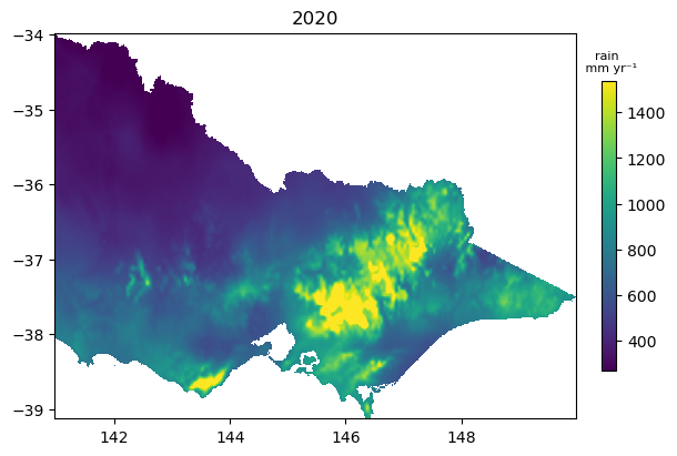
Plot annual data
Below we resample the climate data into an annual series. As we have loaded rainfall in the default example, we calculate an annual sum. This statistic may not make sense if you are loading a different variable, e.g. temperature.
[6]:
climate_annual = climate.resample(time='1YE').sum()
climate_annual = climate_annual.odc.mask(poly=geom) # need to remask after a sum to remove zeros
/env/lib/python3.10/site-packages/odc/geo/_xr_interop.py:500: UserWarning: grid_mapping=crs is not pointing to valid coordinate
  warnings.warn(
[7]:
fig, ax = plt.subplots(figsize=(6, 4), layout='constrained')

im = climate_annual.isel(time=0).plot(cmap='viridis', add_labels=False, robust=True, add_colorbar=False, ax=ax)
ax.set_title(climate_annual.isel(time=0).time.dt.year.item())

cb = fig.colorbar(im, ax=ax, shrink=0.75, orientation='vertical')
cb.ax.set_title(var + ' \n mm yr\u207B\u00B9', fontsize=8);
Section 2: ECMWF Reanalysis v5 (ERA5)
We can also load ERA5 reanalysis datasets using Google’s collection of Analysis-Ready, Cloud Optimized ERA5 data. ERA5 has a coarse spatial resolution (~25 km) compared with ANUClim, but provides hourly reconstructions of past climate and has many more climate fields at both surface and pressure levels.
A list of variables to load is available in the data summary table. Some commonly used long and short variable names are the following: * 2 metre temperature : 2t * total_precipitation : tp * 2m_dewpoint_temperature : 2d * evaporation : e * 10m_u_component_of_wind : 10u * 10m_v_component_of_wind : 10v *
Surface short-wave (solar) radiation downwards : ssrd
Analysis parameters for ERA5
era5_var: Provide a variable name to loadtime_range: length of time to load
[8]:
era5_var = 'total_precipitation'
time_range = ('2020-01-01', '2020-12-31')
Open a dask client
This helps with ERA5 data as it has a larger volume of time steps to summarise.
[9]:
create_local_dask_cluster()
Client
Client-421a5cbe-6110-11f0-8194-a257d99bdb0e
| Connection method: Cluster object | Cluster type: distributed.LocalCluster |
| Dashboard: /user/chad.burton@ga.gov.au/proxy/8787/status |
Cluster Info
LocalCluster
ca9e844b
| Dashboard: /user/chad.burton@ga.gov.au/proxy/8787/status | Workers: 1 |
| Total threads: 2 | Total memory: 15.00 GiB |
| Status: running | Using processes: True |
Scheduler Info
Scheduler
Scheduler-05038069-2097-41e3-92b4-66463e14f10b
| Comm: tcp://127.0.0.1:38757 | Workers: 1 |
| Dashboard: /user/chad.burton@ga.gov.au/proxy/8787/status | Total threads: 2 |
| Started: Just now | Total memory: 15.00 GiB |
Workers
Worker: 0
| Comm: tcp://127.0.0.1:41071 | Total threads: 2 |
| Dashboard: /user/chad.burton@ga.gov.au/proxy/44255/status | Memory: 15.00 GiB |
| Nanny: tcp://127.0.0.1:44099 | |
| Local directory: /tmp/dask-scratch-space/worker-ptuthvpu | |
Define a function for loading ERA5
[10]:
def load_era5(
    x=None,
    y=None,
    crs="EPSG:4326",
    time=None,
    bands=None,
    chunks=None,
    path="gs://gcp-public-data-arco-era5/ar/full_37-1h-0p25deg-chunk-1.zarr-v3",
):
    # Lazily load Zarr from Google Cloud Platform
    era5_ds = xr.open_zarr(path, chunks=chunks, storage_options=dict(token="anon"))

    # Select bands
    era5_ds = era5_ds[bands] if bands is not None else era5_ds

    # Clip to extent
    if x is not None:
        bbox = BoundingBox.from_xy(x, y, crs=crs).to_crs(crs)
        era5_ds = era5_ds.sel(
            longitude=slice(bbox.left, bbox.right),
            latitude=slice(bbox.top, bbox.bottom),
        )

    # Select time
    if time is not None:
        era5_ds = era5_ds.sel(time=slice(time[0], time[-1]))

    return era5_ds.odc.assign_crs(crs)
Convert the polygon back to EPSG:4326
[11]:
# convert our vector back to EPSG 4326 for ERA5
gdf = gdf.to_crs('epsg:4326')

# define bounding box of the geometry
# we'll use this to select data before masking
bb = gdf.total_bounds
Load total precipitation
[12]:
era5_climate = load_era5(
    x=(bb[0],bb[2]),
    y=(bb[1],bb[3]),
    crs="EPSG:4326",
    time=time_range,
    bands=[era5_var],
    chunks=dict(x=10, y=10, time=2000), # really small chunks
    path="gs://gcp-public-data-arco-era5/ar/full_37-1h-0p25deg-chunk-1.zarr-v3",
)

era5_climate = era5_climate[era5_var]
era5_climate
[12]:
<xarray.DataArray 'total_precipitation' (time: 8784, latitude: 21, longitude: 36)> Size: 27MB
dask.array<getitem, shape=(8784, 21, 36), dtype=float32, chunksize=(2000, 21, 36), chunktype=numpy.ndarray>
Coordinates:
  * latitude     (latitude) float32 84B -34.0 -34.25 -34.5 ... -38.75 -39.0
  * longitude    (longitude) float32 144B 141.0 141.2 141.5 ... 149.5 149.8
  * time         (time) datetime64[ns] 70kB 2020-01-01 ... 2020-12-31T23:00:00
    spatial_ref  int32 4B 4326
Attributes:
    long_name:   Total precipitation
    short_name:  tp
units: mResample to annual
As ERA5 has an hourly time step, we need to use dask to resample into annual time fields as there is a lot of data even though the spatial extent of the subset of data is small. This can take a few minutes on the default sandbox.
[13]:
era5_climate_annual = era5_climate.resample(time='1YE').sum().load()
Mask with the polygon
[14]:
geometry = gdf.iloc[0].geometry
geom = Geometry(geom=geometry, crs=gdf.crs)
era5_climate_annual = era5_climate_annual.odc.mask(poly=geom) # need to remask after a sum to remove zeros
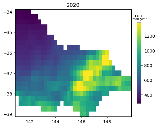
Plot an annual summary data
[15]:
fig, ax = plt.subplots(figsize=(5, 4), layout='constrained')

im = (era5_climate_annual*1000).isel(time=0).plot(cmap='viridis', add_labels=False, robust=True, add_colorbar=False, ax=ax);  # multiply by 1000 to convert into mm
ax.set_title(era5_climate_annual.isel(time=0).time.dt.year.item())

cb = fig.colorbar(im, ax=ax, shrink=0.75, orientation='vertical')
cb.ax.set_title(var + ' \n mm yr\u207B\u00B9', fontsize=8);
Additional information
License: The code in this notebook is licensed under the Apache License, Version 2.0. Digital Earth Australia data is licensed under the Creative Commons by Attribution 4.0 license.
Contact: If you need assistance, please post a question on the Open Data Cube Discord chat or on the GIS Stack Exchange using the open-data-cube tag (you can view previously asked questions here). If you would like to report an issue with this notebook, you can file one on
GitHub.
Last modified: April 2025
Compatible datacube version:
[16]:
print(datacube.__version__)
1.8.19
Tags
Tags: NCI compatible, sandbox compatible, :index:`precipitation, air temperature, external data, climate data, downloading data, no_testing