Masking data using the Fmask cloud mask 
Sign up to the DEA Sandbox to run this notebook interactively from a browser
Compatibility: Notebook currently compatible with both the
NCIandDEA SandboxenvironmentsProducts used: ga_ls8c_ard_3
Background
In the past, remote sensing researchers would reject partly cloud-affected scenes in favour of cloud-free scenes. However, multi-temporal analysis techniques increasingly make use of every quality assured pixel within a time series of observations. The capacity to automatically exclude low quality pixels (e.g. clouds, shadows or other invalid data) is essential for enabling these new remote sensing methods.
Analysis-ready satellite data from Digital Earth Australia includes pixel quality information that can be used to easily “mask” data (i.e. keep only certain pixels in an image) to obtain a time series containing only clear or cloud-free pixels.
Description
In this notebook, we show how to mask Digital Earth Australia satellite data using boolean masks. The notebook demonstrates how to:
Load in a time series of satellite data including the
fmaskpixel quality bandInspect the band’s
flags_definitionattributesCreate clear and cloud-free masks and apply these to the satellite data
Buffer cloudy/shadowed pixels by dilating the masks by a specified number of pixels
Clean cloudy/shadowed pixels to reduce false positive cloud detection
Mask out invalid nodata values and replace them with
nan
Getting started
First we import relevant packages and connect to the datacube. Then we define our example area of interest and load in a time series of satellite data.
[1]:
import scipy.ndimage
import xarray
import numpy
import datacube
from datacube.utils.masking import make_mask
from datacube.utils.masking import mask_invalid_data
from odc.algo import mask_cleanup

import sys
sys.path.insert(1, '../Tools/')
from dea_tools.plotting import rgb
Connect to the datacube
[2]:
dc = datacube.Datacube(app="Masking_data")
Create a query and load satellite data
To demonstrate how to mask satellite data, we will load Landsat 8 surface reflectance RGB data along with a pixel quality classification band called fmask.
Note: The
fmaskpixel quality band contains categorical data. When loading this kind of data, it is important to use a resampling method that does not alter the values of the input cells. In the example below, we resamplefmaskdata using the “nearest” method which preserves its original values. For all other bands with continuous values, we use “average” resampling.
[3]:
# Create a reusable query
y, x = -31.492482, 115.610186
radius = 0.03
query = {
"x": (x - radius, x + radius),
"y": (y - radius, y + radius),
"time": ("2015-07", "2015-10")
}
# Load data from the Landsat 8 satellite
data = dc.load(product="ga_ls8c_ard_3",
measurements=["nbart_blue", "nbart_green", "nbart_red", "fmask"],
output_crs="EPSG:3577",
resolution=[-30, 30],
resampling={
"fmask": "nearest",
"*": "bilinear"
},
group_by='solar_day',
**query)
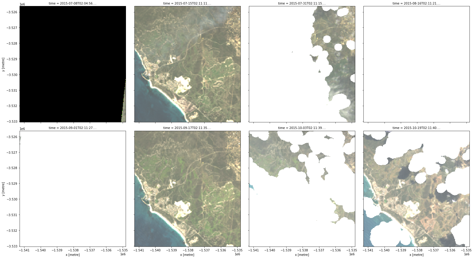
# Plot the data
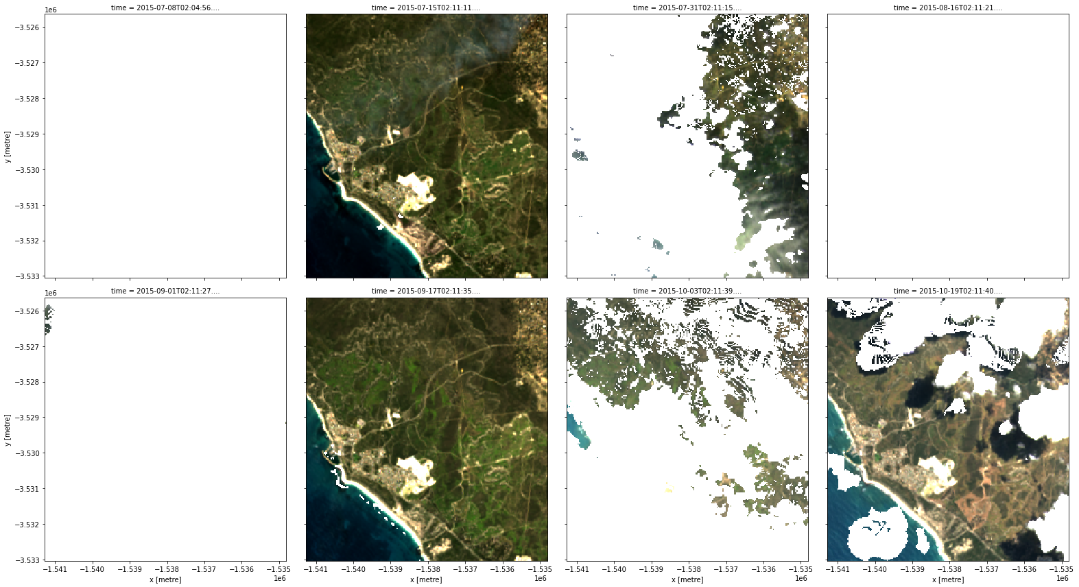
rgb(data, col="time")
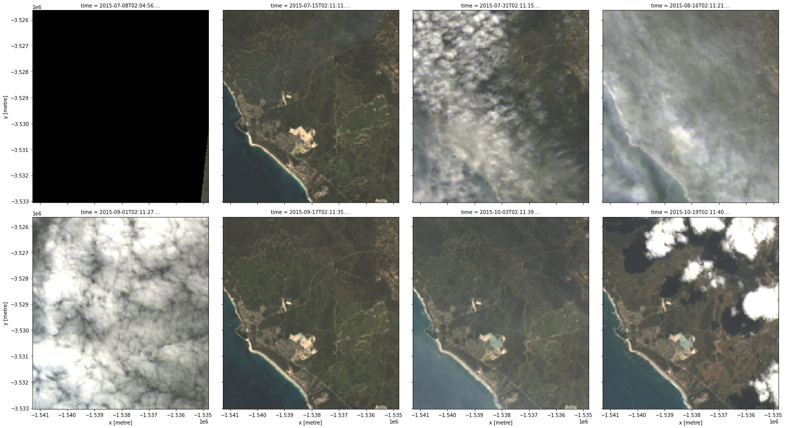
These images show that our area of interest partially crosses the edge of the satellite track (e.g. the first panel), and therefore some areas in the image have no observed data. By inspecting our first timestep, we see that the nodata attribute reports the value -999, and that some of the pixels have that value:
[4]:
data.nbart_red.isel(time=0)
[4]:
<xarray.DataArray 'nbart_red' (y: 247, x: 216)>
array([[-999, -999, -999, ..., -999, -999, -999],
       [-999, -999, -999, ..., -999, -999, -999],
       [-999, -999, -999, ..., -999, -999, -999],
       ...,
       [-999, -999, -999, ...,  430,  420,  393],
       [-999, -999, -999, ...,  396,  388,  378],
       [-999, -999, -999, ...,  442,  396,  376]], dtype=int16)
Coordinates:
    time         datetime64[ns] 2015-07-08T02:04:56.777964
  * y            (y) float64 -3.526e+06 -3.526e+06 ... -3.533e+06 -3.533e+06
  * x            (x) float64 -1.541e+06 -1.541e+06 ... -1.535e+06 -1.535e+06
    spatial_ref  int32 3577
Attributes:
    units:         1
    nodata:        -999
    crs:           EPSG:3577
grid_mapping: spatial_refWe can find the classification scheme of the fmask band in its flags definition:
[5]:
data.fmask.attrs["flags_definition"]
[5]:
{'fmask': {'bits': [0, 1, 2, 3, 4, 5, 6, 7],
  'values': {'0': 'nodata',
   '1': 'valid',
   '2': 'cloud',
   '3': 'shadow',
   '4': 'snow',
   '5': 'water'},
  'description': 'Fmask'}}
[6]:
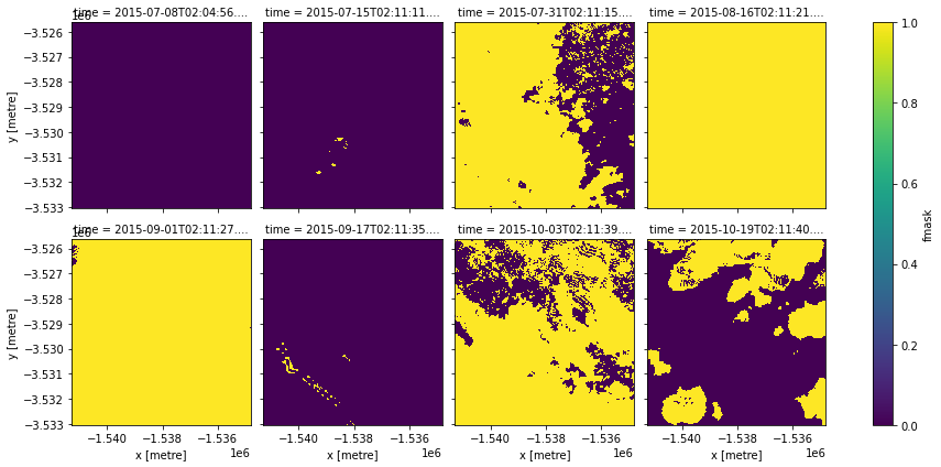
data.fmask.plot(col="time", col_wrap=4)
[6]:
<xarray.plot.facetgrid.FacetGrid at 0x7fef0e59bfa0>
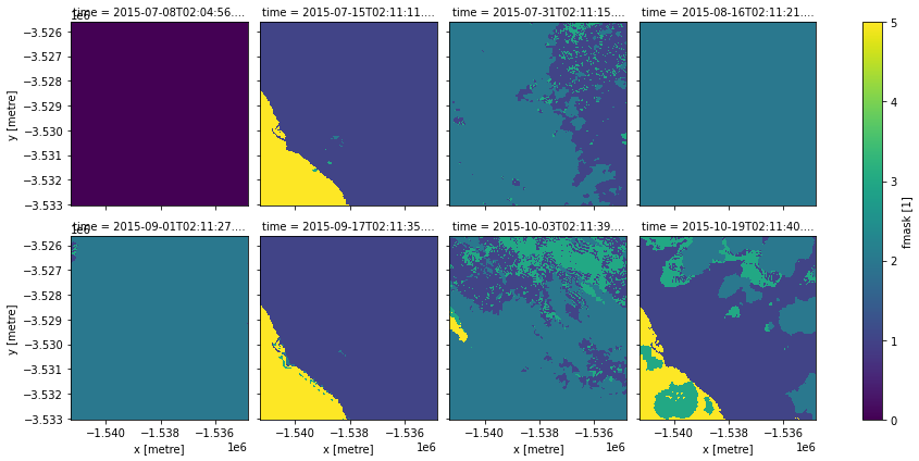
We see that fmask also reports the nodata pixels, and along with the cloud and shadow pixels, it picked up the ocean as water too.
Cloud-free images
Creating the clear-pixel mask
We create a mask by specifying conditions that our pixels must satisfy. But we will only need the labels (e.g. fmask="valid") to create a mask.
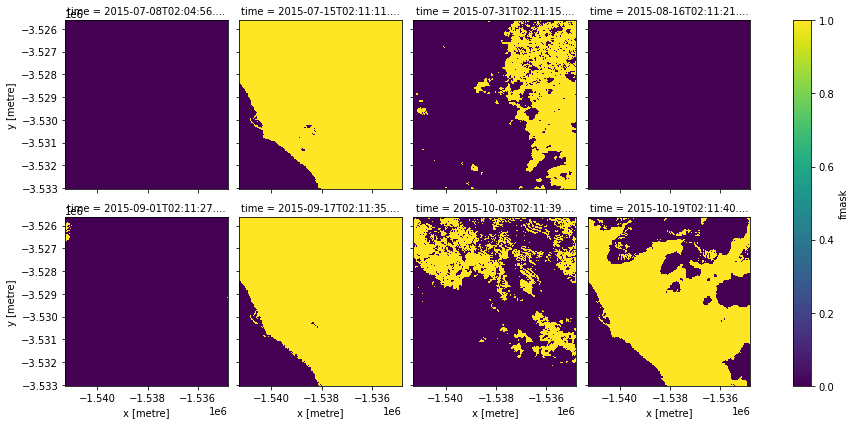
[7]:
# Create the mask based on "valid" pixels
clear_mask = make_mask(data.fmask, fmask="valid")
clear_mask.plot(col="time", col_wrap=4)
[7]:
<xarray.plot.facetgrid.FacetGrid at 0x7fef0e8a8520>
Applying the clear-pixel mask
We can now get the clear images we want.
[8]:
# Apply the mask
clear = data.where(clear_mask)
rgb(clear, col="time")
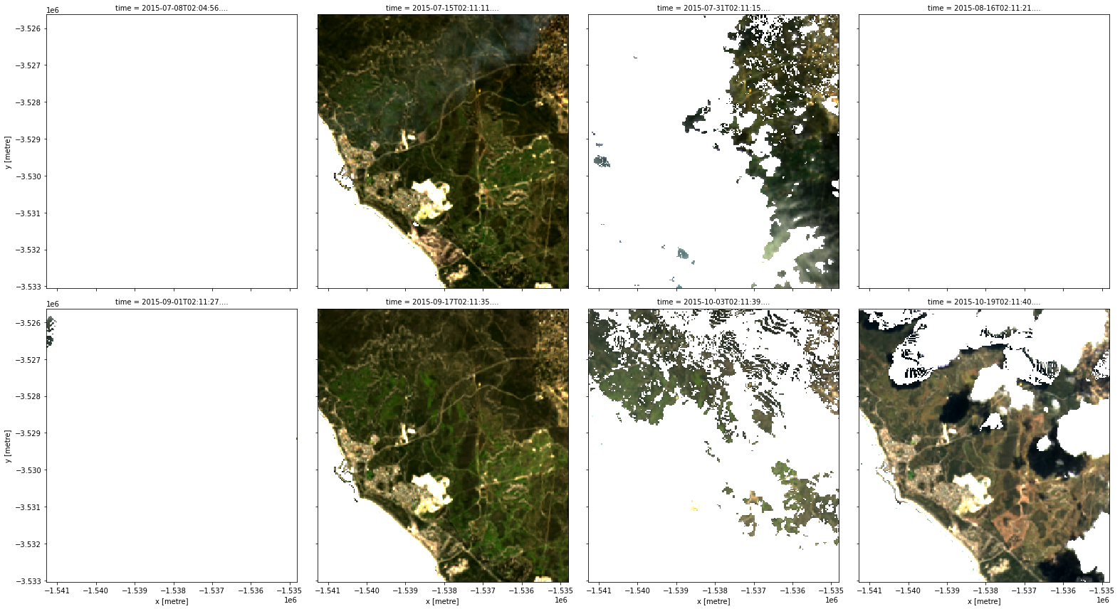
Cloud-free images
If we look carefully, we can see that we have lost the ocean too. Sometimes we may instead want to create a mask using a combination of different fmask features. For example, below we create a mask that will preserve pixels that are flagged as either valid, water or snow (and mask out any cloud or cloud shadow pixels):
[9]:
# Identify pixels that are either "valid", "water" or "snow"
cloud_free_mask = (
    make_mask(data.fmask, fmask="valid") |
    make_mask(data.fmask, fmask="water") |
    make_mask(data.fmask, fmask="snow")
)

# Apply the mask
cloud_free = data.where(cloud_free_mask)
rgb(cloud_free, col="time")
Mask dilation and cleaning
Sometimes we want our cloud masks to be more conservative and mask out more than just the pixels that fmask classified as cloud or cloud shadow. That is, sometimes we want a buffer around the cloud and the shadow. We can achieve this by dilating the mask using the mask_cleanup function from odc.algo.
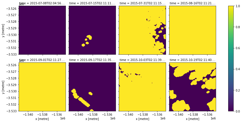
Because we now want to focus on cloud and cloud shadow pixels, we first do the opposite to our previous examples and create a mask which has True values if a pixel contains either cloud or cloud shadow, and False for all others (e.g. valid, snow, water). When we plot this data, cloud and cloud shadow will appear as yellow, and other pixels as purple.
[10]:
# Identify pixels that are either "cloud" or "cloud_shadow"
cloud_shadow_mask = (
    make_mask(data.fmask, fmask="cloud") |
    make_mask(data.fmask, fmask="shadow")
)

# Plot
cloud_shadow_mask.plot(col="time", col_wrap=4)
[10]:
<xarray.plot.facetgrid.FacetGrid at 0x7fef0c199be0>
We now apply mask_cleanup. This function allows us to modify areas of cloud and cloud shadow using image processing techniques called morphological operations. These tools can be used to expand and contract regions of our image to change the shape of specific features - in this case, clouds and cloud shadow. Four of the most useful morphological
techniques include:
Dilation: Expand (i.e. “dilate”)
Truevalues outward, resulting in largerTruefeaturesErosion: Shrink (i.e. “erode”)
Truevalues inward, resulting in smallerTruefeaturesClosing: First dilate, then erode
Truepixels. This is used to fill small or narrowFalsegaps inside or betweenTruefeatures.Opening: First erode, then dilate
Truepixels. This is used to remove small or narrow areas ofTruefeatures, but preserve larger features.
All of these operations are applied using a specific radius to control how many pixels our clouds and shadows are dilated, eroded, closed or opened. For example, we can specify that our clouds and shadows are expanded by 5 pixels in all directions as follows:
[11]:
# Dilate all cloud and cloud shadow pixels by 5 pixels in all directions
cloud_shadow_buffered = mask_cleanup(mask=cloud_shadow_mask,
                                     mask_filters=[("dilation", 5)])
cloud_shadow_buffered.plot(col="time", col_wrap=4)
[11]:
<xarray.plot.facetgrid.FacetGrid at 0x7feef9b65e50>
Our clouds and shadows (yellow) have now been expanded outwards (compare this to the cloud_shadow_mask data we plotted earlier).
We can now apply this dilated cloud and shadow mask to our original data (note we need to reverse our mask using ~ so that valid pixels are marked with True as in our original un-dilated example).
[12]:
# Apply the mask
buffered_cloud_free = data.where(~cloud_shadow_buffered)
rgb(buffered_cloud_free, col="time")
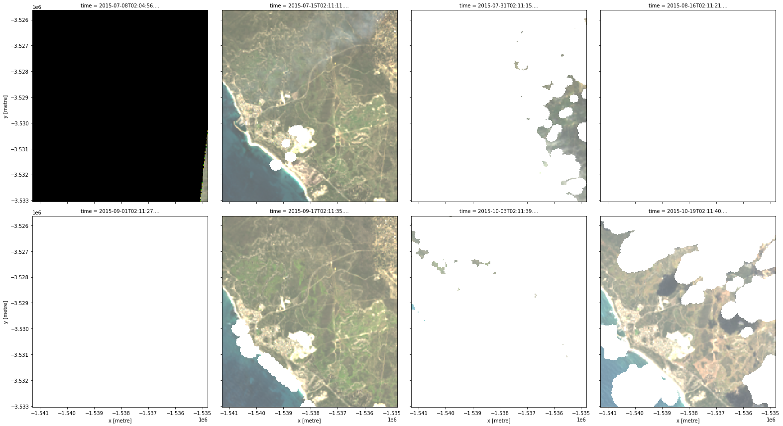
Cloud mask data from fmask can commonly include false positive clouds over features including urban areas, bright sandy beaches and salt pans. We can see an example of this in the sixth panel, where a length of beach has been erroneously mapped as cloud.
To reduce these false positives, it can often be useful to apply a morphological “opening” operation before we dilate our clouds and shadows. This operation can remove small or narrow clouds by first “shrinking” then “expanding” our cloud and shadow pixels. To apply an opening operation with a radius of 3, we can supply an extra ("opening", 3) processing step using mask_cleanup:
[13]:
# Dilate all cloud and cloud shadow pixels by 5 pixels in all directions
cloud_shadow_buffered = mask_cleanup(mask=cloud_shadow_mask,
                                     mask_filters=[("opening", 3), ("dilation", 5)])

# Apply the mask
buffered_cloud_free = data.where(~cloud_shadow_buffered)
Now when we plot our data, we can see that the sixth panel is no longer affected by false positive clouds along the bright narrow beach.
Note: Morphological operations and radiuses are application-specific; make sure to experiment with a range of options to make sure they have the effect you are looking for.
[14]:
rgb(buffered_cloud_free, col="time")
Masking out invalid data
Finally, we need to set all pixels containing -999 nodata values to nan so that they do not affect subsequent analyses. This can be performed automatically using the mask_invalid_data function:
[15]:
# Set invalid nodata pixels to NaN
valid_data = mask_invalid_data(buffered_cloud_free)
rgb(valid_data, col='time')
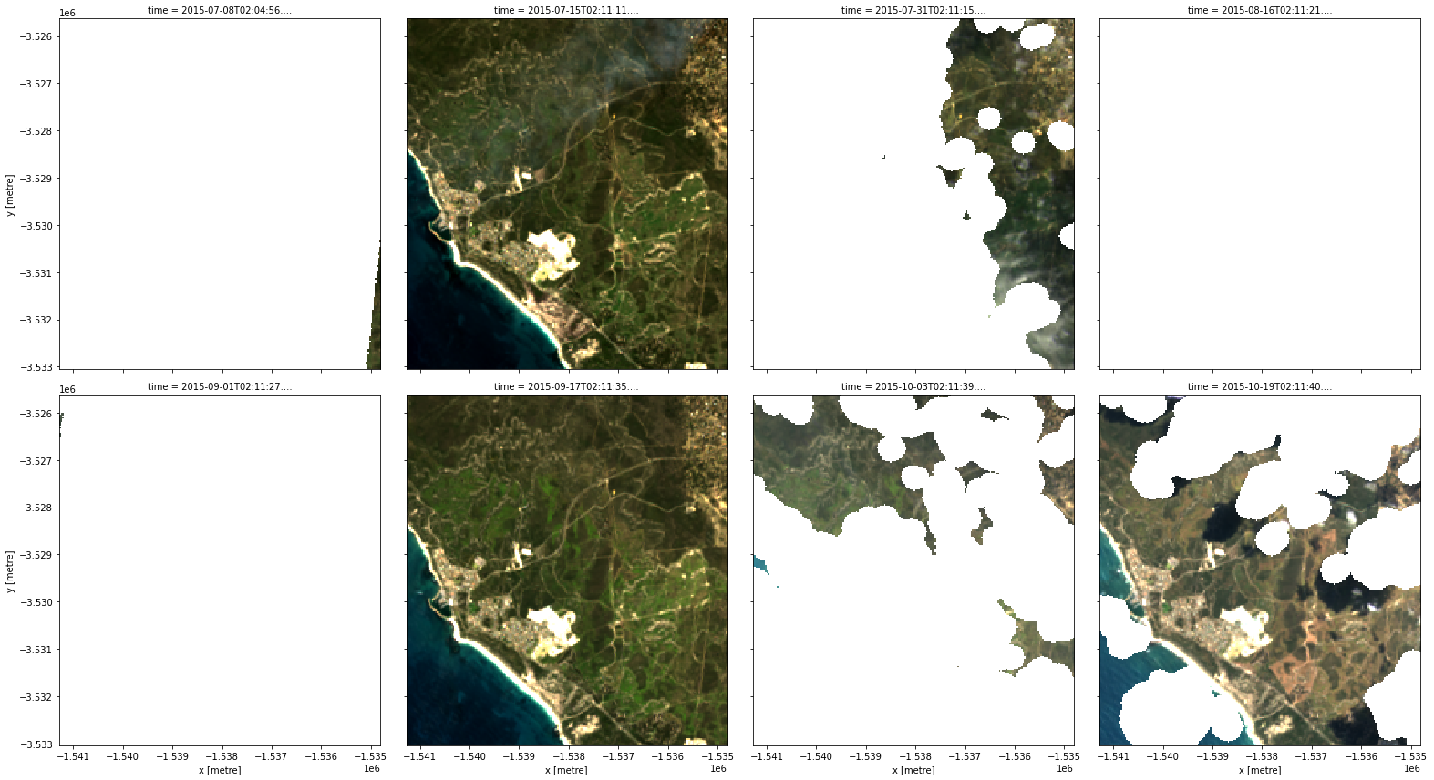
When we inspect our data, we can see that all -999 values have now been replaced with nan:
[16]:
valid_data.nbart_red.isel(time=0)
[16]:
<xarray.DataArray 'nbart_red' (y: 247, x: 216)>
array([[ nan,  nan,  nan, ...,  nan,  nan,  nan],
       [ nan,  nan,  nan, ...,  nan,  nan,  nan],
       [ nan,  nan,  nan, ...,  nan,  nan,  nan],
       ...,
       [ nan,  nan,  nan, ..., 430., 420., 393.],
       [ nan,  nan,  nan, ..., 396., 388., 378.],
       [ nan,  nan,  nan, ..., 442., 396., 376.]])
Coordinates:
    time         datetime64[ns] 2015-07-08T02:04:56.777964
  * y            (y) float64 -3.526e+06 -3.526e+06 ... -3.533e+06 -3.533e+06
  * x            (x) float64 -1.541e+06 -1.541e+06 ... -1.535e+06 -1.535e+06
    spatial_ref  int32 3577
Attributes:
    units:         1
    nodata:        -999
    crs:           EPSG:3577
grid_mapping: spatial_refAdditional information
License: The code in this notebook is licensed under the Apache License, Version 2.0. Digital Earth Australia data is licensed under the Creative Commons by Attribution 4.0 license.
Contact: If you need assistance, please post a question on the Open Data Cube Discord chat or on the GIS Stack Exchange using the open-data-cube tag (you can view previously asked questions here). If you would like to report an issue with this notebook, you can file one on
GitHub.
Last modified: December 2023
Compatible datacube version:
[17]:
print(datacube.__version__)
1.8.6
Tags
Tags: sandbox compatible, NCI compatible, sentinel 2, dea_plotting, dea_datahandling, rgb, dilate, masking, cloud masking, buffering