Extracting random samples from xarray.DataArray

Sign up to the DEA Sandbox to run this notebook interactively from a browser
Compatibility: Notebook currently compatible with both the NCI and DEA Sandbox environments
Products used: ga_ls_landcover_class_cyear_3, ga_ls8cls9c_gm_cyear_3

Description

This notebook introduces an efficient and highly scalable python function: dea_tools.validation.xr_random_sampling(), for extracting random pixel samples from a classified xarray.DataArray. Random sampling is a fundamental step when preparing reference data and is commonly used in remote sensing workflows, whether for validating classification outputs or extracting training samples for supervised learning tasks.

The sampling function introduced here supports a range of stratification strategies, including:

Stratified random sampling: draws random samples from each class, proportional to class size—useful when preserving class distribution is important.
Equal stratified random sampling: samples an equal number of points from each class, helping to balance imbalanced datasets and reduce classifier bias.
Manual per-class sampling: allows users to specify the number of samples per class, offering fine-grained control.
Simple random: draw simple random samples across an array, regardless of class distributions.

Choosing the right sampling strategy depends on the analysis goals. For example, equal stratified sampling may improve classifier robustness when classes are imbalanced, while proportional sampling might better suited when real-world class frequencies for validation statistics are required.

This notebook will load a classified dataset from the DEA Land Cover product, and use the xr_random_sampling() function to extract samples using all of the sampling strategies listed above.

Load packages

Import Python packages that are used for the analysis

[1]:

import datacube
import matplotlib.pyplot as plt
from odc.geo.xr import assign_crs
from matplotlib.colors import ListedColormap

import sys
sys.path.insert(1, "../Tools/")
from dea_tools.validation import xr_random_sampling
from dea_tools.landcover import lc_colourmap, get_colour_scheme, make_colourbar

Connect to the datacube

Connect to the datacube so we can access DEA data.

[2]:

dc = datacube.Datacube(app="Random_sampling")

Analysis parameters

central_lat: Central latitude for the study area (e.g. -35.29). Set this to the approximate centre of your area of interest.
central_lon: Central longitude for the study area (e.g. 149.113). Set this to the approximate centre of your area of interest.
buffer: Distance in degrees to load around the central point (e.g. 0.3). Controls the size of the spatial bounding box—larger buffers will load a bigger area and may increase processing time.
time: Time range for analysis as a tuple of start and end dates in YYYY-MM-DD format (e.g. ("2023-01-01", "2023-12-31")).

[3]:

# Set the central latitude and longitude
central_lat = -34.819
central_lon =  138.699

# Set the buffer to load around the central coordinates.
buffer = 0.3

#time range to load
time = ("2023-01-01", "2023-12-31")

# Compute the bounding box for the study area
latitude = (central_lat - buffer, central_lat + buffer)
longitude = (central_lon - buffer, central_lon + buffer)

Load DEA Land Cover data

We will also load a geomedian from the same period for visualisation purposes.

[4]:

# Load DEA Land Cover data
lc = dc.load(
    product="ga_ls_landcover_class_cyear_3",
    output_crs="EPSG:3577",
    measurements=["level3"],
    x=longitude,
    y=latitude,
    resolution=(-30, 30),
    time=time,
)

# Convert to datarray and mask any no-data
lc = lc["level3"].squeeze()
lc = lc.where(lc != 255)

# Also load a geomedian
ds = dc.load(
    product="ga_ls8cls9c_gm_cyear_3",
    time=time,
    measurements=["nbart_red", "nbart_green", "nbart_blue"],
    x=longitude,
    y=latitude,
    output_crs="EPSG:3577",
    resolution=(30, -30),
).squeeze()

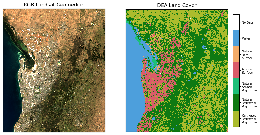
Plot DEA Land Cover and RGB imagery

[5]:

fig, ax = plt.subplots(1, 2, figsize=(11, 5.5), sharey=True)

ds[["nbart_red", "nbart_green", "nbart_blue"]].to_array().plot.imshow(
    robust=True, ax=ax[0], add_labels=False
)
ax[0].set_title("RGB Landsat Geomedian")
ax[0].axes.get_xaxis().set_ticks([])
ax[0].axes.get_yaxis().set_ticks([])

colour_scheme = get_colour_scheme("level3")
cmap, norm = lc_colourmap(colour_scheme)
im = lc.plot(cmap=cmap, norm=norm, ax=ax[1], add_labels=False, add_colorbar=False)
make_colourbar(fig, ax[1], measurement="level3", labelsize=7, horizontal=False)

ax[1].set_title("DEA Land Cover")
ax[1].axes.get_xaxis().set_ticks([])
ax[1].axes.get_yaxis().set_ticks([]);

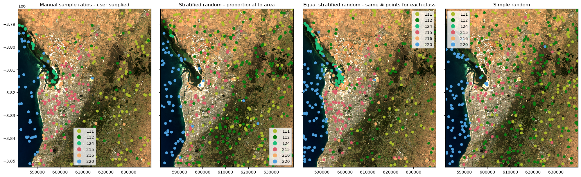
../../../_images/notebooks_How_to_guides_Random_sampling_11_0.png

Extract random samples from DEA Land Cover

Using the different sampling strategies outlined in the Description section above.

[6]:

# Manual samples per class
print('User defined per-class samples')
train_points_manual = xr_random_sampling(
    lc,
    sampling="manual",
    manual_class_ratios={
        "111": 100,
        "112": 25,
        "124": 25,
        "215": 75,
        "216": 35,
        "220": 40,
    },
)
print('\n')
print('Stratified random samples')

# Stratified random samples
train_points_stratified_random = xr_random_sampling(
    lc, sampling="stratified_random", n=400
)
print('\n')
print('Equal stratified random samples')

# Equal stratified random samples
train_points_equal_stratified_random = xr_random_sampling(
    lc, sampling="equal_stratified_random", n=400
)
print('\n')
print('Simple random samples')

# Simple random samples
train_points_random = xr_random_sampling(lc, sampling="random", n=400)

User defined per-class samples
Class 111: sampling 100 points
Class 112: sampling 25 points
Class 124: sampling 25 points
Class 215: sampling 75 points
Class 216: sampling 35 points
Class 220: sampling 40 points


Stratified random samples
Class 111: sampling 129 points
Class 112: sampling 163 points
Class 124: sampling 3 points
Class 215: sampling 39 points
Class 216: sampling 5 points
Class 220: sampling 61 points


Equal stratified random samples
Class 111: sampling 67 points
Class 112: sampling 67 points
Class 124: sampling 67 points
Class 215: sampling 67 points
Class 216: sampling 67 points
Class 220: sampling 67 points


Simple random samples
Sampling 400 points

Plot the samples

Plotting the samples over the geomedian map will provide context for the sample locations.

[7]:

fig, ax = plt.subplots(1, 4, figsize=(20, 6), sharey=True, layout="constrained")

# Trim no-data off the colormap
cmap=ListedColormap(cmap.colors[:-1])

ds[["nbart_red", "nbart_green", "nbart_blue"]].to_array().plot.imshow(
    robust=True, ax=ax[0], add_labels=False)
train_points_manual.plot(ax=ax[0], column="class", cmap=cmap, legend=True, categorical=True)
ax[0].set_title("Manual sample ratios - user supplied")

ds[["nbart_red", "nbart_green", "nbart_blue"]].to_array().plot.imshow(
    robust=True, ax=ax[1], add_labels=False)
train_points_stratified_random.plot(ax=ax[1], column="class", cmap=cmap, legend=True, categorical=True)
ax[1].set_title("Stratified random - proportional to area")

ds[["nbart_red", "nbart_green", "nbart_blue"]].to_array().plot.imshow(
    robust=True, ax=ax[2], add_labels=False)
train_points_equal_stratified_random.plot(ax=ax[2], column="class", cmap=cmap, legend=True, categorical=True)
ax[2].set_title("Equal stratified random - same # points for each class")

ds[["nbart_red", "nbart_green", "nbart_blue"]].to_array().plot.imshow(
    robust=True, ax=ax[3], add_labels=False)
train_points_random.plot(ax=ax[3], column="class", cmap=cmap, legend=True, categorical=True)
ax[3].set_title("Simple random");

../../../_images/notebooks_How_to_guides_Random_sampling_15_0.png

Sampling extremely large rasters

One of the key features of xr_random_sampling is its ability to extract samples from extremely large rasters while still efficiently managing memory.

When a given class in a raster contains fewer than one billion samples (pixels), the function will create a mask of where all pixels match a given class, and then randomly sample the class using numpy.random.choice. However, when the number of samples exceeds one billion, to reduce memory usage, the function will instead randomly sample a subset of all pixel coordinates and check which ones match the target class. To reduce the chance of undersampling, the parameter oversample_factor controls how many candidate coordinates are initially drawn. For example, if 100 samples are required and oversample_factor=5, 500 random (x, y) coordinates will be sampled first. Only those matching the class will be retained and then randomly sub-sampled down to the desired number of samples. If too few valid matches are found, a warning is issued. Increasing the oversample_factor value can improve success rates when sampling sparse or spatially fragmented classes in large datasets, at the cost of more memory and computation.

In the example below, we load DEA Land Cover over the Australian continent at 60 metre resolution, this results in ~4.4 billion float32 pixels (float because we mask the 255 no-data values). When extracting samples using the equal_stratified_random method, the function uses 30-40 GiB of RAM and takes about 5-6 mins to complete.

We include an example below as markdown text only because this example uses too much memory for a small machine like the DEA Sandbox, but if you have access to a larger machine you can test it out yourself.

Sampling DEA Landcover over the entire Australian Continent

# Load DEA Land Cover over whole continent
lc = dc.load(
    product="ga_ls_landcover_class_cyear_3",
    output_crs="EPSG:3577",
    measurements=[
        "level3",
    ],
    resolution=(-60, 60),
    time=time
)

lc = lc['level3'].squeeze()
lc = lc.where(lc!=255)

print('total pixels =', len(lc.x)*len(lc.y))

# Extract random samples with large oversample factor
train_points_equal_stratified_random = xr_random_sampling(
    lc, sampling="equal_stratified_random", n=3000, oversample_factor=10
)

# Plot the samples
fig, ax = plt.subplots(1, 1, figsize=(8, 7))

train_points_equal_stratified_random.plot(
    ax=ax,
    column="class",
    cmap=cmap,
    categorical=True,
    legend=True,
)

ax.set_title("Equal stratified random - same n-points for each class")
ax.axes.get_xaxis().set_ticks([])
ax.axes.get_yaxis().set_ticks([]);

$image.png$

Additional information

License: The code in this notebook is licensed under the Apache License, Version 2.0. Digital Earth Australia data is licensed under the Creative Commons by Attribution 4.0 license.

Contact: If you need assistance, please post a question on the Open Data Cube Discord chat or on the GIS Stack Exchange using the open-data-cube tag (you can view previously asked questions here). If you would like to report an issue with this notebook, you can file one on GitHub.

Last modified: July 2025

Compatible datacube version:

[8]:

print(datacube.__version__)

1.8.19