Creating a Wetlands Insight Tool stacked line plot 
Sign up to the DEA Sandbox to run this notebook interactively from a browser
Compatibility: Notebook currently compatible with the
DEA SandboxenvironmentProducts used: DEA Wetlands Insight Tool
Background
Wetlands provide a wide range of ecosystem services including improving water quality, carbon sequestration, as well as providing habitat for fish, amphibians, reptiles and birds.
The Digital Earth Australia Wetlands Insight Tool (DEA WIT) summarises variations in the amount of water, green vegetation, dry vegetation and bare soil over time in wetlands, providing users with the ability to compare past and present wetland behaviours. It achieves this by combining DEA data products DEA Water Observations, DEA Tasseled Cap Wetness Percentiles and DEA Fractional Cover, all derived from Landsat satellite imagery, as a stacked line plot showing changes in wetland cover type over time.
Expected output
This code-free interactive notebook demonstrates the method for reproducing results from the Wetlands Insight Tool. At the end of the notebook you will display and save a WIT plot (Figure 1).
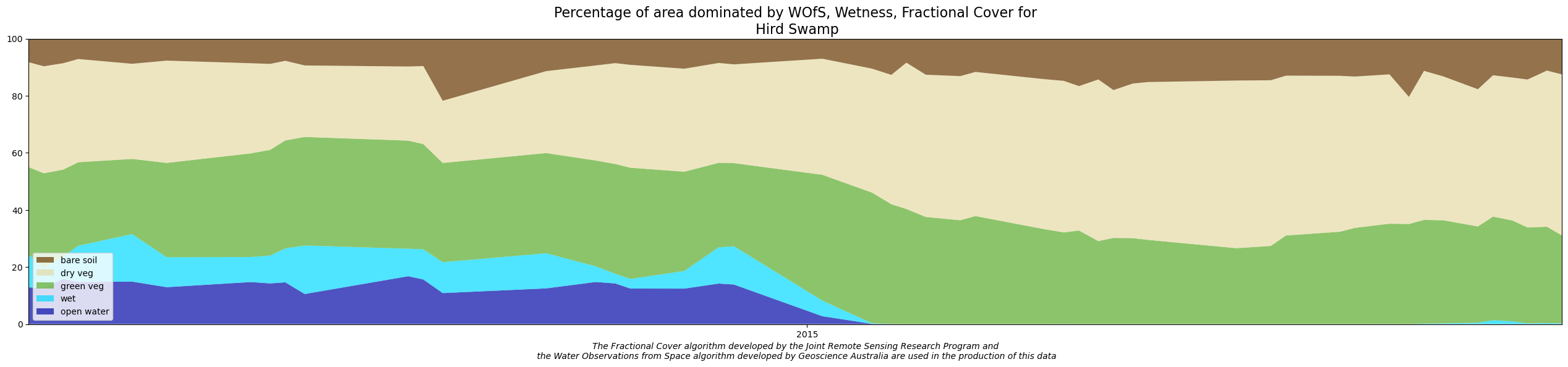
Figure 1 Stacked line plot of Hird Swamp, Victoria showing open water (dark blue), wet as defined by tasseled cap wetness (light blue), green vegetation (green), dry vegetation (light brown), and bare soil (dark brown). Each of these components are shown as a percentage of the area of the polygon.
Description
This notebook demonstrates how to use the WIT interactive app to analyse a wetland of interest by generating a stacked line plot (Figure 1). The plot visualises changes in open water, wet (mixed water and vegetation), green vegetation, dry vegetation and bare soil over time by representing the relative proportion of each class inside the wetland area at each step of the timeseries.
The interactive app allows users to draw a polygon on the map to assess wetland changes over recent decades. Alternatively, existing wetland boundaries in shapefile or GeoJSON format can be uploaded directly. Results can be exported as both visual figures and raw CSV files containing the WIT data for a selected time period since 1987.
An advanced option includes generating Spatial WIT which is a spatial representation of the classifications used in the Wetlands Insight Tool. See Dunn et al., 2023 and DEA Wetlands Insight Tool notebook to understand the caveats. Users should note also that the water and wet classes are binary and the vegetation fractional cover classes are percentages per pixel, with the spatial representation scaled accordingly (Figure 2).
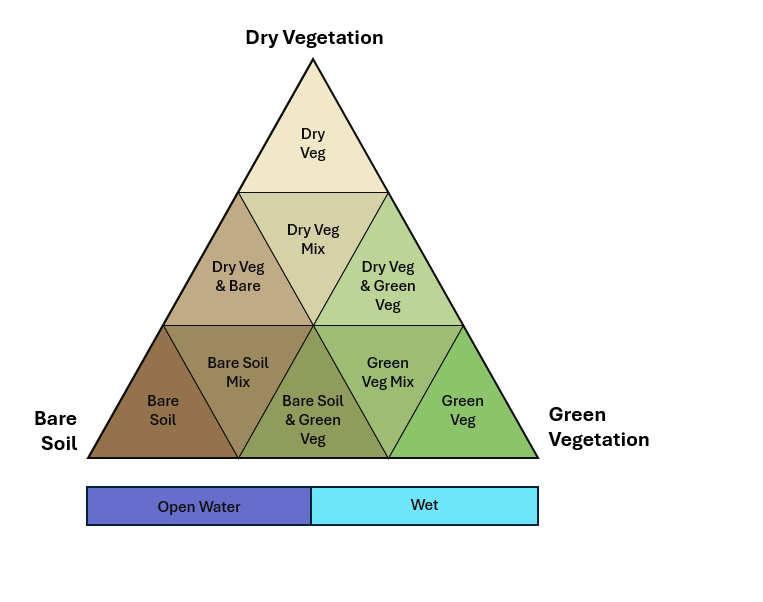
Figure 2: Ternary diagram depicting fractional cover composition, where each vertex represents a pure end-member: green vegetation, dry vegetation, and bare soil. The plot is subdivided into smaller triangles, representing varying mixtures of these three components, with proportions summing to 100%.
No coding experience is required to use the app.
Note: Before using the DEA Wetlands Insight Tool it is important to understand its limitations. This information, as well as other technical details, are outlined in the official Geoscience Australia DEA Wetlands Insight Tool product description. For a more in depth explanation of the method used to generate the stacked line plots, refer to the DEA Wetlands Insight Tool notebook.
Getting started
To run this analysis, run all the cells in the notebook, starting with the “Load packages” cell. From the upper notebook menu and toolbar, either press the ▶️ button in each code cell or select the Run dropdown menu and select Run All Cells.
Load packages
[1]:
import sys

sys.path.insert(1, "../Tools/")
from dea_tools.app import wetlandsinsighttool
/env/lib/python3.10/site-packages/distributed/node.py:187: UserWarning: Port 8787 is already in use.
Perhaps you already have a cluster running?
Hosting the HTTP server on port 36717 instead
  warnings.warn(
Client
Client-697d9268-6052-11f0-87bc-328c65a8c342
| Connection method: Cluster object | Cluster type: distributed.LocalCluster |
| Dashboard: /user/lauren.schenk@ga.gov.au/proxy/36717/status |
Cluster Info
LocalCluster
ebcd1451
| Dashboard: /user/lauren.schenk@ga.gov.au/proxy/36717/status | Workers: 1 |
| Total threads: 2 | Total memory: 12.21 GiB |
| Status: running | Using processes: True |
Scheduler Info
Scheduler
Scheduler-feb176de-31ec-46ac-b4a3-e99395e3902e
| Comm: tcp://127.0.0.1:41219 | Workers: 1 |
| Dashboard: /user/lauren.schenk@ga.gov.au/proxy/36717/status | Total threads: 2 |
| Started: Just now | Total memory: 12.21 GiB |
Workers
Worker: 0
| Comm: tcp://127.0.0.1:42815 | Total threads: 2 |
| Dashboard: /user/lauren.schenk@ga.gov.au/proxy/45167/status | Memory: 12.21 GiB |
| Nanny: tcp://127.0.0.1:39211 | |
| Local directory: /tmp/dask-scratch-space/worker-3y8wcyag | |
DEA Wetlands Insight Tool stacked line plot app
This app provides a code-free mechanism to enable you to interactively draw a polygon around any Australian wetland of interest and generate a WIT stacked line plot to explore changes in the behaviour of the wetland over time. To use the tool:
Follow the Getting started instructions to run the
wetlandsinsighttool.wit_app()cell below to initiate the interactive application.On the left of the map, enter the name of your wetland into
Wetland Name. This will be used in the title of the WIT plot and output file names. A.csvwill be exported with this app.Zoom in on the map and use the
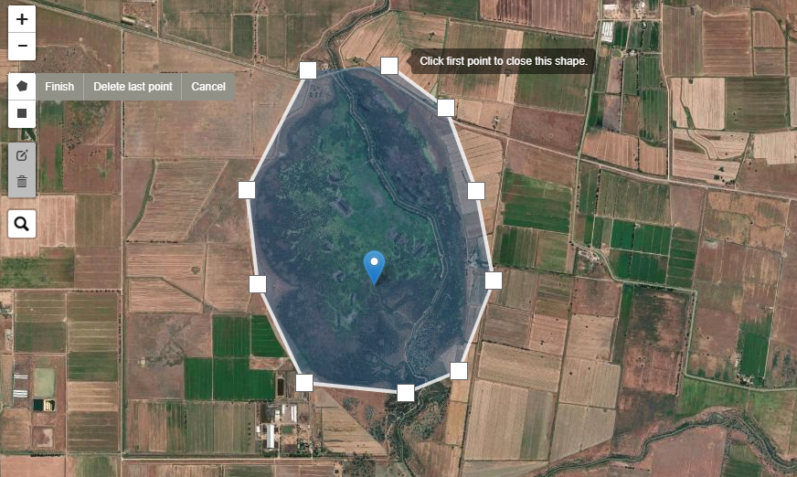
Draw a polygonorDraw a rectangletools on the left of the map to draw a shape around your wetland, as per the figure below. > Note: > - To keep load times reasonable, the app is restricted to areas smaller than 2,000 square kilometres in size. After drawing your polygon, look for theTotal polygon areain the top of the app. For areas greater than this, processing times may be extremely slow or will cease altogether. > - A GeoJSON of your drawn shape will automatically be exported. You can reuse this shape in subsequent runs using the step below. To download the shape for use between sandbox sessions, you’ll need to right click the file in the file menu and selectDownload. Your wetland shape file will be namedtest_drawn_polygon.geojsonand you can also rename the file by right clicking on it. To reuse the file in later sandbox sessions, it can be re-loaded into the app by selecting the ↥Uploadicon in the app.
Alternatively to drawing a polygon, a shapefile or GeoJSON containing a wetland polygon can be uploaded using the ↥
Uploadbutton in the app (uploaded files should be less than 5 megabytes in size). > Note: Ensure that uploaded files contain only 2D polygon geometries with no “z” dimension/coordinates. If this is not the case, “z” coordinates will need to be removed before the interactive app can be run.When you are ready, press the
Runbutton on the bottom left to begin extracting the stacked line plot. During processing, status updates will appear below the map. When processing is complete, the WIT plot will appear below the status updates and the output files will appear in the/Interactive_apps/file menu. Patience may be required during data processing of WIT plots and spatial animations. > Optional: Tick theFigure (.png)box to export the WIT plot as a.pngimage.
[2]:
wetlandsinsighttool.wit_app()
[2]:
Advanced settings
This interactive tool includes advanced features that can be accessed by clicking the Advanced tab in the menu to the left of the map:
Override maximum size limit: Allows users to override the default 2,000 square kilometre area limit. This enables analysis of larger wetland areas but should be used with caution, as it may cause memory issues or crashes.Spatial WIT animation: Generates the spatial WIT animation as a.gifalong with associated.tifand.pngfiles for each frame within the animation. All.tifand.pngoutputs will be saved to a new folder in this directory calleddeawetlands_outputs.
Important: Be careful when running the Spatial WIT animation multiple times as your storage in the Sandbox can fill up. It is advised you download the outputs you desire after each run and delete all outputs in the deawetlands_outputs folder regularly.
Next steps: Wetlands Insight Tool notebook
The DEA Wetlands Insight Tool notebook in this repository provides more details about the method used to generate the WIT stacked line plot. Run this notebook if you would like to see the code behind the plots.
Additional information
Citations — To cite this notebook’s dataset in your work you can attribute the following publications:
Dunn, B., Ai, E., Alger, M.J., Fanson, B., Fickas, K.C., Krause, C.E., Lymburner, L., Nanson, R., Papas, P., Ronan, M., Thomas, R.F., 2023. Wetlands Insight Tool: Characterising the Surface Water and Vegetation Cover Dynamics of Individual Wetlands Using Multidecadal Landsat Satellite Data. Wetlands 43, 37. Available: https://doi.org/10.1007/s13157-023-01682-7
Krause, C., Dunn, B., Bishop-Taylor, R., Adams, C., Burton, C., Alger, M., Chua, S., Phillips, C., Newey, V., Kouzoubov, K., Leith, A., Ayers, D., Hicks, A., DEA Notebooks contributors 2021. Digital Earth Australia notebooks and tools repository. Geoscience Australia, Canberra. Available: https://doi.org/10.26186/145234
Contact: If you need assistance, please post a question on the Open Data Cube Discord chat or on the GIS Stack Exchange using the open-data-cube tag (you can view previously asked questions here). If you would like to report an issue with this notebook, you can file one on
GitHub.
Last modified: March 2025
Compatible datacube versions
[3]:
import datacube

print(datacube.__version__)
1.8.19