Model and customise intertidal exposure 
Sign up to the DEA Sandbox to run this notebook interactively from a browser
Compatibility: Notebook currently compatible with the
DEA SandboxenvironmentProducts used: ga_s2ls_intertidal_cyear_3, ga_ls8cls9c_gm_cyear_3
Background
Intertidal exposure
Intertidal coastlines support a wide array of habitats and coastal and marine species. Low energy tidal flats often support mangrove and seagrass habitats which in turn play host to sea birds, mammals and reptiles. Tropical and subtropical intertidal coral reefs provide habitat, food and shelter. Soft sediment coastlines support microphytobenthos and intertidal algae are ubiquitously distributed across Australia.
The combined effects of tide, sun and air make intertidal environments one of the most dynamic places for life on Earth. Consequently, ecological niches exist within these environments where optimal conditions vary over timescales that range from daily to seasonally and beyond. Seagrass, coral and algae, for instance, all experience decline under varying combinations of exposure with season, solar irradiance and air temperature. Intertidal exposure characteristics and the prevalence of these species in intertidal habitats can further influence the presence and distribution of other intertidal occupying species, such as seabirds and dugongs.
Intertidal exposure describes the amount of time that intertidal areas are exposed to air from tide coverage. Leveraging intertidal elevation mapping, the exposure calculation translates high temporal resolution tidal modelling to determine percentage exposure times for intertidal regions, at 10 m2 resolution. Exploiting the local influences of tidal harmonic inputs into global tidal modelling, intertidal exposure mapping can tease out exposure patterns over temporal scales such as daytime, nighttime or season.
Mapping the exposure dynamics of intertidal areas and contrasting their patterns of change over varying timescales supports our ability to further characterise and understand intertidal habitats. Supporting an array of important marine species, it also offers insights into how exposure patterns influence species behaviours and distributions over short (month to season) to long (multi-annual) timescales.
Description
This notebook outlines the general methodology required to calculate intertidal exposure and demonstrates how tailored calculations can be used to investigate specific temporal influences on exposure times in intertidal ecosystems.
In this notebook, users will: 1. Use a conceptual model to understand how the intertidal exposure calculation is derived. 2. Through the use of case studies, calculate:
- Full exposure characteristics
- Seasonally filtered exposure characteristics
- Combined seasonal and daily exposure characteristics
- Inverted exposure to calculate monthly, night time inundation characteristics
Introduction to the intertidal exposure calculation method
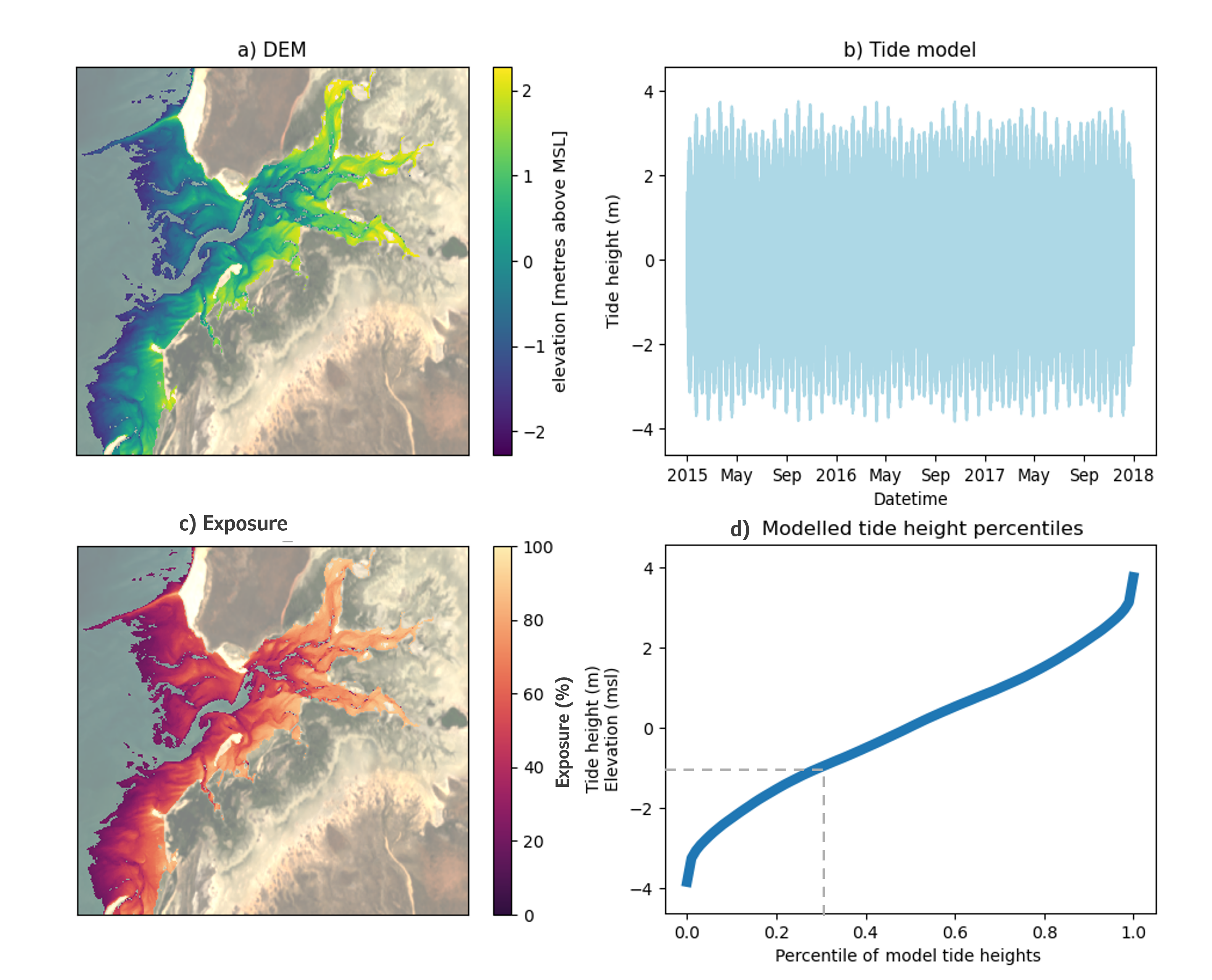
DEA Intertidal Exposure models the percentage of time that any intertidal pixel of known elevation is exposed from tidal inundation. Exposure is calculated by comparing the pixel elevation back against a high temporal resolution model of tide heights for that location. Exposure percentage represents the proportion of tidally exposed observations (those lower than the pixel elevation) relative to the total number of tide model observations, generated for the 3-year product epoch.
This is demonstrated in the figure below where panel a shows the digital elevation model for Carnot Bay in Western Australia, produced for the three year epoch centered around 2016. A tide model was generated at 30 minute time intervals for the same temporal epoch (panel b) and is summarised in the cumulative distribution curve in panel d. For computational efficiency, a single tide height model is generated to represent the entire area of interest (panel a). Additionally, modelled tide heights and intertidal elevations are mapped to the same datum - meters above mean sea level (msl). Intertidal exposure (panel c) is calculated for every elevation value (y-axis panel d) as the equivalent percentile distribution of modelled tide heights (x-axis, panel d). This equates to the fraction of all modelled tides that were exposed per elevation during the modelled epoch and is used as a proxy for time, where:
Exposure Elevation z = Tide height percentile * 100 %
In panel d, this is demonstrated by the grey-dashed line, where
Exposure -1.0 msl =0.3 * 100 = 30 %
In other words, 30 % of tide heights, modelled at 30 min intervals between 1 Jan 2015 and 31 Dec 2017 (panel b), occur at or below intertidal elevations of -1.0 msl, meaning this elevation is exposed from inundation for 30 % of the modelled time period.
Custom filtering of the intertidal exposure calculation
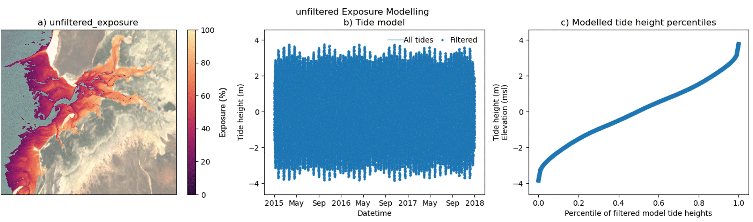
In addition to modelling exposure for a full time period, the exposure algorithm supports filtering of selected time periods from within the epoch. This enables the exploration of exposure dynamics across a range of custom time periods, including day, night, month and season as well as combinations of time periods, e.g. Daytime-Summer exposure. Users should note that the exposure calculation is performed against a single all-epoch time elevation model of the area of interest.
The animated figure below demonstrates the effect on exposure (panel a) of filtering time periods of interest from within the tidal model (panel b) on the resultant percentile tide height curve (panel c). Temporal filtering of the exposure model exploits natural changes in the local tide model, influenced by tidal harmonics, local bathymetry and the relative position of the Earth to the moon and sun. The effect of temporal filtering on the exposure maps (panel a) is most pronounced at the upper and lower ends of the modelled tide height range (panel c). Local tide modelling varies widely across Australian coastlines and so the impact of these end-member influences will vary with location. Furthermore, satellite biases in high and low tide image acquisition for some locations may also produce gaps in the modelling of intertidal elevation as well as exposure at these extreme ends of the tide range. Caused by the sun-synchronous orbits of the sensors used to capture baseline datasets in these models, offsets in the imaging of extreme tide heights are mapped in the DEA Intertidal data suite and are demonstrated in a following section of this notebook.
Getting started
To run this analysis, start with the “Load packages” cell. Using the “Run” menu at the top of the page, select “Run All Cells”.
To edit this analysis for your own area of interest, update the parameters in the “Analysis parameters” cell below. Rename the study_area parameter and replace the x and y coordinates for diagonally opposite latitude and longitude pairs in your area of interest, using the WGS84/EPSG:4326 coordinate reference system. For support using other coordinate reference systems, see the DEA Notebooks Beginners Guide. To find your coordinates, we
recommend using DEA Maps. To change the annual summary views, look for documented directions to update the time parameter throughout the analysis.
Load packages
Import Python packages that are used for the analysis.
[1]:
# Install some non-default functionality
!pip install git+https://github.com/GeoscienceAustralia/dea-intertidal.git@772a95c
!pip install sunriset
Collecting git+https://github.com/GeoscienceAustralia/dea-intertidal.git@772a95c
  Cloning https://github.com/GeoscienceAustralia/dea-intertidal.git (to revision 772a95c) to /tmp/pip-req-build-yt9jnb1p
  Running command git clone --filter=blob:none --quiet https://github.com/GeoscienceAustralia/dea-intertidal.git /tmp/pip-req-build-yt9jnb1p
  WARNING: Did not find branch or tag '772a95c', assuming revision or ref.
  Running command git checkout -q 772a95c
  Resolved https://github.com/GeoscienceAustralia/dea-intertidal.git to commit 772a95c
  Preparing metadata (setup.py) ... done
Requirement already satisfied: sunriset in /env/lib/python3.10/site-packages (1.0)
Requirement already satisfied: pytz in /env/lib/python3.10/site-packages (from sunriset) (2024.1)
Requirement already satisfied: pandas in /env/lib/python3.10/site-packages (from sunriset) (2.2.3)
Requirement already satisfied: numpy>=1.22.4 in /env/lib/python3.10/site-packages (from pandas->sunriset) (1.26.4)
Requirement already satisfied: python-dateutil>=2.8.2 in /env/lib/python3.10/site-packages (from pandas->sunriset) (2.9.0)
Requirement already satisfied: tzdata>=2022.7 in /env/lib/python3.10/site-packages (from pandas->sunriset) (2024.2)
Requirement already satisfied: six>=1.5 in /env/lib/python3.10/site-packages (from python-dateutil>=2.8.2->pandas->sunriset) (1.16.0)
If you encounter any issues running the following cell after this install step, consider restarting the kernel. From the top menu, select Kernel then Restart Kernel... and continue running the notebook from the following cell.
[2]:
import datacube
import cmocean
import glob
import os
import numpy as np
import xarray as xr
import imageio.v2 as imageio
import matplotlib.pyplot as plt
from IPython.display import Image
from IPython import display
from IPython.core.display import Video
from ipywidgets import Output, GridspecLayout

import odc.geo.xr
from datacube.utils.cog import write_cog
from datacube.utils.masking import mask_invalid_data
from dea_tools.plotting import display_map, xr_animation, rgb

from intertidal.exposure import exposure
Connect to the DEA datacube
Connect to the DEA database. The app parameter is unique to the analysis in this notebook.
[3]:
# Connect to the datacube to access DEA data.
dc = datacube.Datacube(app='Customising_Intertidal_Exposure')
Load data
The following cells will: * connect to the DEA datacube, * identify and show the analysis parameters, * load satellite and intertidal data for an area of interest, and * plot the outputs as maps, summary graphs and animations
The default area of interest for this analysis is Queensland’s Smithburne River mouth which flows into the eastern side of the Gulf of Carpentaria. Its vast and dynamic intertidal area forms part of the extensive East Asian-Australasian Flyway for migratory seabirds in the Gulf of Carpentaria. Recognised as a wetland of national significance, it is also a region that hosts significant patches of seagrass and supports a wide variety of marine fauna populations.
Analysis parameters
The Smithburne River is used here to demonstrate how various calculations of intertidal exposure can reveal insights into intertidal environments. Once you have run this notebook through start to finish, try editing the study area and coordinates in the cell below to explore your own small area of interest.
study_area: Location name (e.g."Gladstone_Harbour")query_params: Parameters to define the total area and period of interesty: Latitude coordinates (e.g.(-23.74437, -23.78851)). Decimal degree coordinates for the diagonnally opposite corners of your area of interestx: Longitude coordinates (e.g.(151.24299, 151.32091)). Decimal degree coordinates for the diagonnally opposite corners of your area of interest (corresponding to corners used fory)time: Analysis period (e.g.("2016", "2022")). A single year or pair of years between which, allDEA Intertidaldatasets will be returned. Note: data can only be requested annually from 2016 onwards.
freq: The temporal frequency used to generate the modelled tide heights (e.g. “2 H” or “30 min”). For computational efficiency, we have nominated a 2 hour frequency for this workbook. For research applications, we recommend a higher frequency, e.g. 30 minutes. Higher frequencies come at the expense of a slower compute time.
[4]:
# Identify your area of interest as degree lat/lon coordinates as well
# your nominated time period as start and end dates. Default times
# range from "2016" to "2022"
study_area = "Smithburne_River_Qld"
query_params = dict(y=(-17.05121, -17.10617),
                    x=(140.90808, 140.97289),
                    time=("2016", "2022"))
freq = "2 H"
# View the area of interest over a generic basemap. Data will be loaded
# inside the red bounding box.
display_map(x=query_params["x"], y=query_params["y"])
[4]:
[5]:
# Load DEA Intertidal for the area of interest, and mask out invalid
# nodata values
ds = dc.load(
    product="ga_s2ls_intertidal_cyear_3",
    measurements=['elevation', 'exposure', 'ta_offset_high','ta_offset_low'],
    **query_params)
ds = mask_invalid_data(ds)

# Load the blended Landsat 8/9 annual geomedian image for
# the area of interest, and mask out invalid nodata values
geomad_ds = dc.load(
    product="ga_ls8cls9c_gm_cyear_3",
    measurements=["nbart_red", "nbart_green", "nbart_blue"],
    resampling="cubic",
    like=ds,
)
geomad_ds = mask_invalid_data(geomad_ds)

# Inspect the combined DEA Intertidal and Geomad dataset
ds
[5]:
<xarray.Dataset> Size: 54MB
Dimensions:         (time: 7, y: 654, x: 734)
Coordinates:
  * time            (time) datetime64[ns] 56B 2016-07-01T23:59:59.999999 ... ...
  * y               (y) float64 5kB -1.85e+06 -1.85e+06 ... -1.857e+06
  * x               (x) float64 6kB 9.495e+05 9.495e+05 ... 9.568e+05 9.569e+05
    spatial_ref     int32 4B 3577
Data variables:
    elevation       (time, y, x) float32 13MB nan nan nan nan ... nan nan nan
    exposure        (time, y, x) float32 13MB nan nan nan nan ... nan nan nan
    ta_offset_high  (time, y, x) float32 13MB 7.0 7.0 7.0 7.0 ... 3.0 3.0 3.0
    ta_offset_low   (time, y, x) float32 13MB 5.0 5.0 5.0 5.0 ... 2.0 2.0 2.0
Attributes:
    crs:           EPSG:3577
grid_mapping: spatial_refPlot and view elevation and exposure for all timesteps
[6]:
# Plot each epoch and save in preparation to animate the time-series
for date in range(0, len(ds.time - 1)):

    # Identify a single timestep to inspect
    time = np.datetime_as_string(ds.time.values, unit="Y")[date]

    # Setup the figure
    fig, axes = plt.subplots(ncols=5, figsize=(20, 4))

    # Assign the datasets to the figure
    rgb(geomad_ds.sel(time=time), bands=["nbart_red", "nbart_green", "nbart_blue"], ax=axes[0])

    rgb(geomad_ds.sel(time=time),
        bands=["nbart_red", "nbart_green", "nbart_blue"],
        ax=axes[1],
        alpha=0.5)
    ds.elevation.sel(time=time).plot(ax=axes[1],
                                     cmap="viridis",
                                     vmin=ds.elevation.min(),
                                     vmax=ds.elevation.max())

    rgb(geomad_ds.sel(time=time),
        bands=["nbart_red", "nbart_green", "nbart_blue"],
        ax=axes[2],
        alpha=0.5)
    ds.exposure.sel(time=time).plot(ax=axes[2],
                                    cmap=cmocean.cm.matter_r,
                                    vmin=0,
                                    vmax=100)

    rgb(geomad_ds.sel(time=time),
        bands=["nbart_red", "nbart_green", "nbart_blue"],
        ax=axes[3],
        alpha=0.5)
    ds.ta_offset_high.sel(time=time).where(
        ds.elevation.sel(time=time).notnull()).plot(
            ax=axes[3],
            cmap="Wistia",
            vmin=0,
            vmax=np.array([ds.ta_offset_high.max(),
                           ds.ta_offset_low.max()]).max() * 2,
        )

    rgb(geomad_ds.sel(time=time),
        bands=["nbart_red", "nbart_green", "nbart_blue"],
        ax=axes[4],
        alpha=0.5)
    ds.ta_offset_low.sel(time=time).where(
        ds.elevation.sel(time=time).notnull()).plot(
            ax=axes[4],
            cmap="Wistia",
            vmin=0,
            vmax=np.array([ds.ta_offset_high.max(),
                           ds.ta_offset_low.max()]).max() * 2,
        )

    labels = [
        f"a) {time} GeoMAD",
        f"b) {time} Intertidal Elevation",
        f"c) {time} Intertidal Exposure",
        f"d) {time} Hightide Offset",
        f"e) {time} Lowtide Offset",
    ]

    for ax, title in zip(axes.reshape(-1), labels):
        ax.tick_params(labelbottom=False,
                       labelleft=False,
                       left=False,
                       bottom=False)
        ax.set(xlabel=None, ylabel=None)
        ax.set_title(title)

    plt.tight_layout()
    plt.savefig(f"{time}_DEA_Intertidal.png")
    plt.close()

# Animate as a gif and view the time-series

# List of images to include in the gif
path = os.getcwd()
image_files = glob.glob(f"{path}/*_DEA_Intertidal.png")
image_files.sort()

# Output path
gif_path = "animated.gif"

# Set the frames per second
fps = 1

# Append each epoch-year as a frame to the gif output
with imageio.get_writer(gif_path, mode="I", fps=fps, loop=0) as writer:
    for file in image_files:
        image = imageio.imread(file)
        writer.append_data(image)

# View the epoch-time gif
Image(gif_path)
[6]:
<IPython.core.display.Image object>
Interpretation
The default Smithburne River, QLD, location is located on the eastern banks of Australia’s Gulf of Carpentaria. A recurved sand spit in this area has been developing over recent decades and is being stabilised by the development of mangrove forest and seagrass tidal flat. The animation above shows annual changes to intertidal area between 2016 and 2022. Panel a shows the location in satellite imagery. Note that the annual median imagery shows approximately median tide levels, disguising much of the intertidal area.
Panels b-e represent some of the intertidal features mapped annually for this location in the DEA Intertidal dataset suite. The intertidal digital elevation model in panel b demonstrates a tide range within approximately +/- 1.5 m above mean sea level. This elevation model is a primary input into the intertidal exposure model (panel c).
Intertidal exposure values represent the percentage of time during the epoch that every 10 m2 pixel was exposed to the air. Although this location appears to represent a fairly complete range of modelled exposure values (%), careful examination shows that extrema values are not captured by this model. This is because there is an offset in satellite image acquisition that fails to capture tide heights at both ends of the tidal spectrum (panels d,e) which gets reflected in the exposure model. Panels d-e show that satellites failed to image this location during the top 3-9 % of high tides (panel d) and during the bottom 0-7 % of low tides (panel e) during the timeseries. These offsets should be kept in mind when interpreting the spatial outputs of any exposure mapping undertaken using this dataset.
Temporally filtered exposure calculation
As demonstrated in the method, intertidal exposure is calculated by comparing tide heights from a high temporal resolution tide model to an intertidal digital elevation model. By filtering out time-periods of interest from the tide model, customised exposure maps can be generated. The following case studies explore this application by mapping single and paired temporal filters to explore the influence of seasonality and solar irradiation on intertidal exposure.
To customise the exposure calculation using temporal filtering, the following options are provided for input into the filters parameter of the exposure function. Calculation of multiple filters is supported by inputting filters as a list. Calculation of paired exposure filters is supported by inputting a list of one or more tuples into the filters_combined parameter of the exposure function, as demonstrated in the later case studies below.
Filters accepted by the exposure algorithm include: * Monthly (e.g. ‘Jan’, ‘Feb’, ‘Mar’ etc) * Austral Season (e.g. ‘Summer’, ‘Autumn’, ‘Winter’ or ‘Spring’) * Equatorial Season (e.g. ‘Dry’ or ‘Wet’) * Solar (e.g. ‘Daylight’ or ‘Night’)
Case study 1 - Mapping exposure by season
Seasonality is a useful way to explore habitat dynamics when considering migratory seabirds. These global travellers migrate from breeding grounds in Siberia and Alaska, through Asia then to Australia to forage, rest and rebuild their energy reserves each year. Arriving in Australia’s north around September, these birds disperse across the country, returning to the north around March where they prepare to return to their Northern Hemisphere breeding grounds.
Migratory seabirds rely heavily on intertidal zones. They are dependent on both the highest elevations to roost and rest and the lowest elevations to forage and feed, preferring best to occupy locations where roosting and foraging grounds are co-located.
This example maps the changing exposure dynamics of intertidal areas by season to investigate its influence on seabird occupation space across the year.
[7]:
# Change the output year by updating `time = time` to `time = '2016'` for example.
# Default is the latest year in the timeseries.
time = time

# Identify the filters to use to identify datetimes of interest from the high resolution tidal model
filters = ["unfiltered", "summer", "autumn", "winter", "spring"]
filters_combined = None

# Calculate Exposure using the filtered dates of interest
exposure_ds, modelledtides_ds = exposure(
    dem=ds.elevation.sel(time=time),
    start_date=str(np.datetime64(time) - np.timedelta64(1, "Y")),
    end_date=str(np.datetime64(time) + np.timedelta64(1, "Y")),
    modelled_freq=freq,
    filters=filters,
    filters_combined=filters_combined,
)

# Add each filtered dataset as a variable in the master dataset 'ds'
for x in list(exposure_ds.keys()):
    ds[f"exposure_{str(x)}"] = exposure_ds[str(x)]

# Separate the variables of interest from the master dataset (ds)
f = ["exposure_unfiltered"]
for e in filters:
    f.append("exposure_" + e)

# View seasonal exposure for a single year
print(f"Mapping seasonal exposure for {time}")

fig = (ds[f].to_array().sel(time=time).plot(col="variable",
                                            cmap=cmocean.cm.matter_r,
                                            vmin=0,
                                            vmax=100,
                                            add_colorbar=False))

for ax, title in zip(fig.axs.flat, f):
    ax.set_title(title)
    ax.label_outer()
    ax.set_xticklabels(labels="")
    ax.set_yticklabels(labels="")
    ax.set_xlabel("")
    ax.set_ylabel("")

fig.add_colorbar(label="Exposure %")
Creating reduced resolution 5000 x 5000 metre tide modelling array
Modelling tides using FES2014 in parallel
/env/lib/python3.10/site-packages/intertidal/exposure.py:381: FutureWarning: 'H' is deprecated and will be removed in a future version, please use 'h' instead.
  time_range = pd.date_range(
100%|██████████| 5/5 [00:33<00:00,  6.70s/it]
Returning low resolution tide array
/env/lib/python3.10/site-packages/rasterio/warp.py:387: NotGeoreferencedWarning: Dataset has no geotransform, gcps, or rpcs. The identity matrix will be returned.
  dest = _reproject(
Filtering timesteps for summer
Filtering timesteps for autumn
Filtering timesteps for winter
Filtering timesteps for spring
Calculating unfiltered exposure
Calculating summer exposure
Calculating autumn exposure
Calculating winter exposure
Calculating spring exposure
Mapping seasonal exposure for 2022
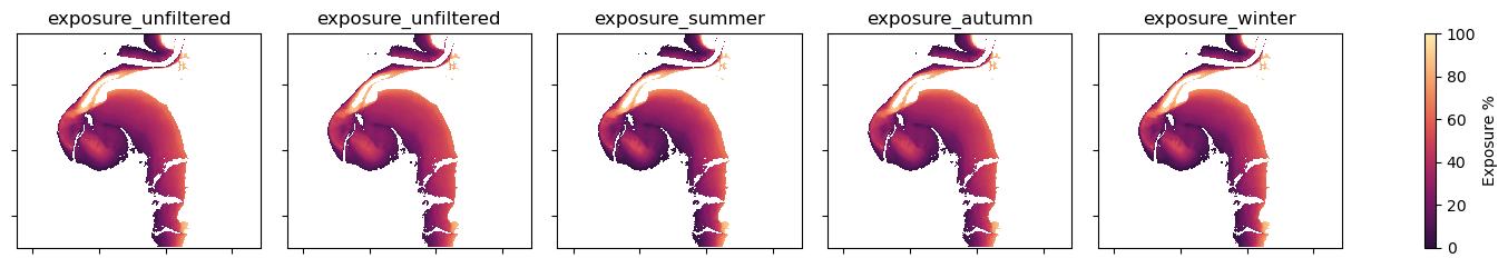
Visual inspection does not notably differentiate these seasonal outputs from one another.
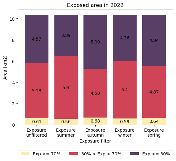
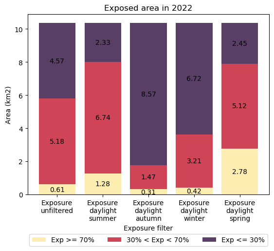
To quantify exposure area across the area of interest, sum the number of pixels into exposure ‘classes’ in the plot below. For simplicity in the plot, we have designated three classes of exposure.
Pixels exposed less than 30 % of the time (approximately low-tide areas)
Pixels exposed between 30 and 70 % of the time (approximately mid-tide areas)
Pixels exposed more than 70 % of the time (approximately high-tide areas)
[8]:
# Explore monthly differences in exposure by area

# Establish some variables to capture the outputs
exp70_100 = []
exp30_70 = []
exp0_30 = []
labels = []

# Separate the exposure datasets into categories and count the pixels per category
for x in ds[f].var():
    if "exp" in x:
        # Prepare the labels for the various exposure datasets
        if x == "exposure":
            labels.append(f"Exposure\nUnfiltered")
        if "exposure_" in x:
            y = x.split("ure_")[-1]
            if "_" in y:
                z = y.split("_")
                labels.append(f"Exposure\n{z[0]}\n{z[-1]}")
            else:
                labels.append(f"Exposure\n{y}")
        # Count the number of pixels exposed between 0 and 100 % of filtered time
        a = ds[str(x)].sel(time=time).count(dim=("x", "y")).values
        # Count the number of pixels exposed between 0 and 70 % of filtered time
        b = (ds[str(x)].sel(time=time).where(ds[str(x)].sel(
            time=time) < 70).count(dim=("x", "y")).values)
        # Count the number of pixels exposed between 0 and 30 % of filtered time
        c = (ds[str(x)].sel(time=time).where(ds[str(x)].sel(
            time=time) <= 30).count(dim=("x", "y")).values)

        # Calculate the pixel counts in each class and translate 10m2 pixel counts to area in km2
        exp70_100.append(round((a[0] - b[0]) * 0.0001, 2))
        exp30_70.append(round((b[0] - c[0]) * 0.0001, 2))
        exp0_30.append(round((c[0]) * 0.0001, 2))

# Prepare the summary data to plot
exp_counts = {
    "Exp >= 70%": (np.array(exp70_100)),
    "30% < Exp < 70%": (np.array(exp30_70)),
    "Exp <= 30%": np.array(exp0_30),
}
# Set the y-axis minimum for this stacked bar chart
bottom = np.zeros(5)
# Set the bar width
width = 0.8
# Set the colour scheme
cmap = cmocean.cm.matter_r
# Prepare the figure
fig, ax = plt.subplots()

# Plot the summary datasets on a stacked bar chart.
for var, counts in exp_counts.items():

    # Set the colour and transparency for each bar
    if var == list(exp_counts.keys())[0]:
        color = cmap(1.0)
        alpha = 1
    if var == list(exp_counts.keys())[1]:
        color = cmap(0.5)
        alpha = 1
    if var == list(exp_counts.keys())[2]:
        color = cmap(0)
        alpha = 0.8
    # Add the bar to the plot
    p = ax.bar(labels,
               counts,
               width,
               label=var,
               bottom=bottom,
               color=color,
               alpha=alpha)
    # Prepare to stack the next bar
    bottom += counts
    # Label each bar with its contribution to the total area
    ax.bar_label(p, label_type="center")

# Prepare the legend
ax.legend(loc="upper center", ncol=3, bbox_to_anchor=(0.5, -0.2), frameon=True)

# Prepare the labels
ax.set_ylabel("Area (km2)")
ax.set_xlabel("Exposure filter")

# Set the figure subtitle
ax.set_title(f"Exposed area in {time}")

plt.show()
Interpretation
Seasonal maps of exposure for this epoch at Smithburne River showed minor differences from the ‘unfiltered’ exposure map. However, assuming the trends are representative of the greater region, this bar-chart summary of exposure extents demonstrates why the area forms part of the important staging grounds for seabird arrivals and departures in Australia.
When migratory seabirds arrive during the Austral spring, they are hungry and energy-depleted. When they depart during Autumn, they are stock piling energy reserves for their return-migration to their breeding grounds. In both cases, they are looking to forage in a location with access to large tidal flats that have accessibility during low tide.
At this Smithburne River location, the largest proportions of low tide foraging grounds (exposed (Exp) less than 30 % of the time) were available during the spring and autumn. Coincidentally, the smallest proportion of low tide foraging ground was available during the Austral summer. Smaller summer foraging grounds may thus be a contributing factor to the continuation of seabird migrations across southern Australia during the warmer months.
Similarly, high tide areas for roosting (exposed for more than 70 % of the time) were also slightly greater during the spring and autumn months.
Case study 2 - Mapping daily exposure by season
In many locations, tidal harmonics, by their very nature, cause differences in absolute day and night time tide heights. Seasonality and the position of the Earth relative to the sun and moon is also a major influence on these diurnal changes in tide height.
This case study uses paired seasonal and daytime filtering of intertidal exposure to explore how intertidal habitats vary across the year. Contextually, intertidal photosynthesisers such as corals (zooxanthellae), seagrasses and algae are all sensitive to the combined effects of solar irradiation and aerial exposure. Paired with annual growing patterns that vary by season, comparing intertidal daytime, seasonal exposure dynamics reveals important insights into the condition and carrying capacities of intertidal habitats across any given year.
[9]:
# Set the year to update data outputs by changing `time = time` to `time = '2016'` for example
time = time

# Identify the paired-filters to use to identify datetimes of interest from the high res tidal model
filters = None
filters_combined = [
    ("daylight", "summer"),
    ("daylight", "autumn"),
    ("daylight", "winter"),
    ("daylight", "spring"),
]

# Use the default settings to calculate a high temporal resolution tide model and
# filter out the nominated datetimes to calculate exposure. Default settings
# include a tide model frequency of 30 minutes
exposure_ds, modelledtides_ds = exposure(
    dem=ds.elevation.sel(time=time),
    start_date=str(np.datetime64(time) - np.timedelta64(1, "Y")),
    end_date=str(np.datetime64(time) + np.timedelta64(1, "Y")),
    modelled_freq=freq,
    filters=filters,
    filters_combined=filters_combined,
)

# Add each filtered dataset as a variable layer in the master dataset 'ds'
for x in list(exposure_ds.keys()):
    ds[f"exposure_{str(x)}"] = exposure_ds[str(x)]

# Separate from the master dataset (ds) the variables of interest
f = ["exposure_unfiltered"]
for e in filters_combined:
    f.append("exposure_" + e[0] + "_" + e[1])

# View the filtered outputs
print(f"Mapping seasonal exposure for {time}")

fig = (ds[f].to_array().sel(time=time).plot(col="variable",
                                            cmap=cmocean.cm.matter_r,
                                            vmin=0,
                                            vmax=100,
                                            add_colorbar=False))

for ax, title in zip(fig.axs.flat, f):
    ax.set_title(title)
    ax.label_outer()
    ax.set_xticklabels(labels="")
    ax.set_yticklabels(labels="")
    ax.set_xlabel("")
    ax.set_ylabel("")

fig.add_colorbar(label="Exposure %")
Creating reduced resolution 5000 x 5000 metre tide modelling array
Modelling tides using FES2014 in parallel
100%|██████████| 5/5 [00:25<00:00, 5.03s/it]
Returning low resolution tide array
Filtering timesteps for daylight
Filtering timesteps for summer
Filtering timesteps for autumn
Filtering timesteps for winter
Filtering timesteps for spring
Calculating unfiltered exposure
Calculating daylight exposure
Calculating summer exposure
Calculating autumn exposure
Calculating winter exposure
Calculating spring exposure
Calculating daylight_summer exposure
Calculating daylight_autumn exposure
Calculating daylight_winter exposure
Calculating daylight_spring exposure
Mapping seasonal exposure for 2022
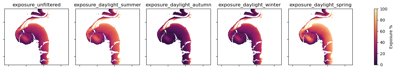
Visual inspection of these exposure maps shows that there are clear differences in the distribution of daytime-seasonally filtered exposure times across a year.
To quantify the changing areas of daytime exposure with season, we will graph grouped pixel counts as previously, using the same classes, as follows:
Pixels exposed less than 30 % of the time (approximately low-tide areas)
Pixels exposed between 30 and 70 % of the time (approximately mid-tide areas)
Pixels exposed more than 70 % of the time (approximately high-tide areas)
[10]:
# Establish some variables to capture the outputs
exp70_100 = []
exp30_70 = []
exp0_30 = []
labels = []

# Separate the exposure datasets into categories and count the pixels per category
for x in ds[f].var():
    if "exp" in x:
        # Prepare the labels for the various exposure datasets
        if x == "exposure":
            labels.append(f"Exposure\nUnfiltered")
        if "exposure_" in x:
            y = x.split("ure_")[-1]
            if "_" in y:
                z = y.split("_")
                labels.append(f"Exposure\n{z[0]}\n{z[-1]}")
            else:
                labels.append(f"Exposure\n{y}")
        # Count the number of pixels exposed between 0 and 100 % of filtered time
        a = ds[str(x)].sel(time=time).count(dim=("x", "y")).values

        # Count the number of pixels exposed between 0 and 70 % of filtered time
        b = (ds[str(x)].sel(time=time).where(ds[str(x)].sel(
            time=time) < 70).count(dim=("x", "y")).values)

        # Count the number of pixels exposed between 0 and 30 % of filtered time
        c = (ds[str(x)].sel(time=time).where(ds[str(x)].sel(
            time=time) <= 30).count(dim=("x", "y")).values)

        # Calculate the pixel count contributions to each class and translate 10m2 pixel counts to area as km2
        exp70_100.append(round((a[0] - b[0]) * 0.0001, 2))
        exp30_70.append(round((b[0] - c[0]) * 0.0001, 2))
        exp0_30.append(round((c[0]) * 0.0001, 2))

# Prepare the summary data to plot

exp_counts = {
    "Exp >= 70%": (np.array(exp70_100)),
    "30% < Exp < 70%": (np.array(exp30_70)),
    "Exp <= 30%": np.array(exp0_30),
}
# Set the y-axis minimum for this stacked bar chart
bottom = np.zeros(5)
# Set the bar width
width = 0.8
# Set the colour scheme
cmap = cmocean.cm.matter_r
# Prepare the figure
fig, ax = plt.subplots()

# Plot the summary datasets on a stacked bar chart.
for var, counts in exp_counts.items():

    # Set the colour and transparency for each bar
    if var == list(exp_counts.keys())[0]:
        color = cmap(1.0)
        alpha = 1
    if var == list(exp_counts.keys())[1]:
        color = cmap(0.5)
        alpha = 1
    if var == list(exp_counts.keys())[2]:
        color = cmap(0)
        alpha = 0.8
    # Add the bar to the plot
    p = ax.bar(labels,
               counts,
               width,
               label=var,
               bottom=bottom,
               color=color,
               alpha=alpha)
    # Prepare to stack the next bar
    bottom += counts
    # Label each bar with its contribution to the total area
    ax.bar_label(p, label_type="center")

# Prepare the legend
ax.legend(loc="upper center", ncol=3, bbox_to_anchor=(0.5, -0.2), frameon=True)

# Prepare the labels
ax.set_ylabel("Area (km2)")
ax.set_xlabel("Exposure filter")

# Set the figure subtitle
ax.set_title(f"Exposed area in {time}")

plt.show()
Interpretation
Daytime exposure mapping by season reveals the dynamicism of intertidal environments in this location across a given year.
Over the Austral autumn and winter at this location, very little intertidal zone was exposed for more than 70 % of the time (0.31 and 0.42 km2 respectively). More than 3/4 of the total intertidal area was exposed for less than 30 % of daylight hours during these cooler seasons. Consequently, these large portions of intertidal area were accustomed to being inundated for long periods during the cooler months.
In the spring and summer seasons, large portions of intertidal area had medium exposure (30 < exp < 70 %) and high exposure (> 70 %), compared to the cooler autumn and winter seasons. Consequently, these areas had greater exposure to the sun and air than cooler seasons (autumn and winter).
These modelled exposure estimates align with field observations related to the stress and mortality of organisms in intertidal zones. For example, Buckee et al (2022) modelled emersion mortality risk in Australian shallow coral reefs and found that across the continent, emersion related coral-mortality risk was generally greatest during the Australian spring time. Causal mechanisms included combinations of mean sea level minima, high incidence of solar irradiation and low daytime air temperatures coinciding with daily exposure periods.
Similarly, seagrass biomass typically peaks around late spring and begins to decline through to winter. Seagrass stress and decline was observed to occur in combination with aerial exposure and maximum daily solar irradiances (e.g. Petrou et al., 2013). Algae also declines under similar conditions, with the addition of temperature being shown to cause dessication and stress during periods of exposure (e.g. Yu et al., 2013).
Spatial and temporal mapping of exposure help to characterise one of the major biophysical influences on species distributions in intertidal habitats. Daytime seasonal exposure mapping is a valuable variable to help explain intertidal species presence and absence across a year.
Case study 3 - Mapping nightly inundation by month
There is a wide range of temporal filtering options that can be used either singly or paired in the intertidal exposure algorithm.
In this case study, we pair night-time and monthly exposure to develop a different understanding of our study site, additionally converting the values from exposure to inundation. To translate exposure (% time) to inundation (% time), simply subtract the exposure value from 100 %. This returns the inverse proportion of modelled tide heights from the cumulative percentile tide-height curve, as demonstrated in the method, representing inundation times as a fraction of the filtered time period.
Contextually, seagrass dependent foragers, such as dugong, source much of their nutritition from shallow intertidal areas. A night-time preference for activity and foraging has been observed in some dugong populations and inundation provides these animals with access to elevated intertidal areas and nutritional sources that deviate from sub-tidal varieties (e.g. Sheppard et al., 2010, Derville et al., 2022). By translating exposure to inundation and mapping the monthly night-time distributions of intertidal inundation, insights into the tidal influences on the presence, absence and distribution of nocturnal intertidal foragers is revealed.
[11]:
# Set the year to update data outputs by changing `time = time` to `time = '2016'` for example
time = time

# Identify the filters to use to identify datetimes of interest from the high res tidal model
filters = None
filters_combined = [
    ("night", "jan"),
    ("night", "feb"),
    ("night", "mar"),
    ("night", "apr"),
    ("night", "may"),
    ("night", "jun"),
    ("night", "jul"),
    ("night", "aug"),
    ("night", "sep"),
    ("night", "oct"),
    ("night", "nov"),
    ("night", "dec"),
]

# Model exposure
exposure_ds, modelledtides_ds = exposure(
    dem=ds.elevation.sel(time=time),
    start_date=str(np.datetime64(time) - np.timedelta64(1, "Y")),
    end_date=str(np.datetime64(time) + np.timedelta64(1, "Y")),
    modelled_freq=freq,
    filters=filters,
    filters_combined=filters_combined,
)

# Separate from the master dataset (ds) the variables of interest
f = ["exposure_unfiltered"]
for e in filters_combined:
    f.append("exposure_" + e[0] + "_" + e[1])

# Add each filtered dataset as a variable layer in the master dataset 'ds'
for x in list(exposure_ds.keys()):
    ds[f"exposure_{str(x)}"] = exposure_ds[str(x)]  # .squeeze(dim='time')

# Calculate the inverse of exposure to convert to inundation
inundation_ds = 100 - exposure_ds

# Separate from the master dataset (ds) the variables of interest
f = ["inundation_unfiltered"]
for e in filters_combined:
    f.append("inundation_" + e[0] + "_" + e[1])

# Add each filtered dataset as a variable layer in the master dataset 'ds'
for x in list(inundation_ds.keys()):
    ds[f"inundation_{str(x)}"] = inundation_ds[str(x)]

# Animate and view the monthly timeseries
# Copy and edit the master dataset
ds2 = ds.sel(time=time)[f].copy(deep=True)
ds2 = ds2.drop_vars(["inundation_unfiltered"])
ds2 = ds2.squeeze("time")

# Reshape the dataset to reset the time dimension for monthly nighttime inundation
variables = [
    ds2[var].expand_dims("time").assign_coords(time=[var])
    for var in ds2.data_vars
]
new_ds = xr.concat(variables, dim="time")
ds2 = new_ds.to_dataset()

newtime = []
for x in range(1, 13, 1):
    if len(str(x)) == 1:
        x = f"0{x}"
    newtime.append(np.datetime64(f"{time}-{x}"))

ds2["time"] = newtime

# Animate and view
xr_animation(
    ds2,
    bands=["inundation_night_jan"],
    output_path=f"{path}_night_inundation.gif",
    interval=1000,
    imshow_kwargs={
        "cmap": cmocean.cm.matter,
        "vmin": 0,
        "vmax": 100
    },
    colorbar_kwargs={"colors": "black"},
    show_text="Inundation %",
    width_pixels=500,
)
plt.close()

# View the monthly, night time inundation gif
Image(f"{path}_night_inundation.gif")
Creating reduced resolution 5000 x 5000 metre tide modelling array
Modelling tides using FES2014 in parallel
100%|██████████| 5/5 [00:26<00:00, 5.33s/it]
Returning low resolution tide array
Filtering timesteps for night
Filtering timesteps for jan
Filtering timesteps for feb
Filtering timesteps for mar
Filtering timesteps for apr
Filtering timesteps for may
Filtering timesteps for jun
Filtering timesteps for jul
Filtering timesteps for aug
Filtering timesteps for sep
Filtering timesteps for oct
Filtering timesteps for nov
Filtering timesteps for dec
Calculating unfiltered exposure
Calculating night exposure
Calculating jan exposure
Calculating feb exposure
Calculating mar exposure
Calculating apr exposure
Calculating may exposure
Calculating jun exposure
Calculating jul exposure
Calculating aug exposure
Calculating sep exposure
Calculating oct exposure
Calculating nov exposure
Calculating dec exposure
Calculating night_jan exposure
Calculating night_feb exposure
Calculating night_mar exposure
Calculating night_apr exposure
Calculating night_may exposure
Calculating night_jun exposure
Calculating night_jul exposure
Calculating night_aug exposure
Calculating night_sep exposure
Calculating night_oct exposure
Calculating night_nov exposure
Calculating night_dec exposure
Exporting animation to /home/jovyan/dev/dea-notebooks/Real_world_examples_night_inundation.gif
[11]:
<IPython.core.display.Image object>
[12]:
# Establish some variables to capture the outputs
inu70_100 = []
inu30_70 = []
inu0_30 = []
labels = []

# Separate the exposure datasets into categories and count the pixels per category
for x in ds[f].var():

    # Prepare the labels for the various exposure datasets
    if x == "inundation_unfiltered":
        labels.append(f"Un-\nfiltered")
    if "inundation_night_" in x:
        y = x.split("night_")[-1]
        if "_" in y:
            z = y.split("_")
            labels.append(f"{z[0]}\n{z[-1]}")
        else:
            labels.append(f"{y}")
    # Count the number of pixels exposed between 0 and 100 % of filtered time
    a = ds[str(x)].sel(time=time).count(dim=("x", "y")).values

    # Count the number of pixels exposed between 0 and 70 % of filtered time
    b = (ds[str(x)].sel(time=time).where(ds[str(x)].sel(time=time) < 70).count(
        dim=("x", "y")).values)

    # Count the number of pixels exposed between 0 and 30 % of filtered time
    c = (ds[str(x)].sel(time=time).where(ds[str(x)].sel(time=time) <= 30).count(
        dim=("x", "y")).values)

    # Calculate the pixel count contributions to each class and translate 10m2 pixel counts to area as km2
    inu70_100.append(round((a[0] - b[0]) * 0.0001, 2))
    inu30_70.append(round((b[0] - c[0]) * 0.0001, 2))
    inu0_30.append(round((c[0]) * 0.0001, 2))

# Prepare the summary data to plot

inu_counts = {
    "Inu >= 70%": (np.array(inu70_100)),  # *0.0001,
    "30% < Inu < 70%": (np.array(inu30_70)),  # *0.0001,
    "Inu <= 30%": np.array(inu0_30),
}  # *0.0001}
# Set the y-axis minimum for this stacked bar chart
bottom = np.zeros(13)
# Set the bar width
width = 0.9
# Set the colour scheme
cmap = cmocean.cm.matter
# Prepare the figure
fig, ax = plt.subplots()

# Plot the summary datasets on a stacked bar chart.
for var, counts in inu_counts.items():

    # Set the colour and transparency for each bar
    if var == list(inu_counts.keys())[0]:
        color = cmap(1.0)
        alpha = 0.8
    if var == list(inu_counts.keys())[1]:
        color = cmap(0.5)
        alpha = 1
    if var == list(inu_counts.keys())[2]:
        color = cmap(0)
        alpha = 1
    # Add the bar to the plot
    p = ax.bar(labels,
               counts,
               width,
               label=var,
               bottom=bottom,
               color=color,
               alpha=alpha)
    # Prepare to stack the next bar
    bottom += counts
    # Label each bar with its contribution to the total area
    ax.bar_label(p, label_type="center")

# Prepare the legend
ax.legend(loc="upper center", ncol=3, bbox_to_anchor=(0.5, -0.2), frameon=True)

# Prepare the labels
ax.set_ylabel("Area (km2)")
ax.set_xlabel("Inundation filter")

# Set the figure subtitle
ax.set_title(f"Night time inundation area in {time}")

plt.show()
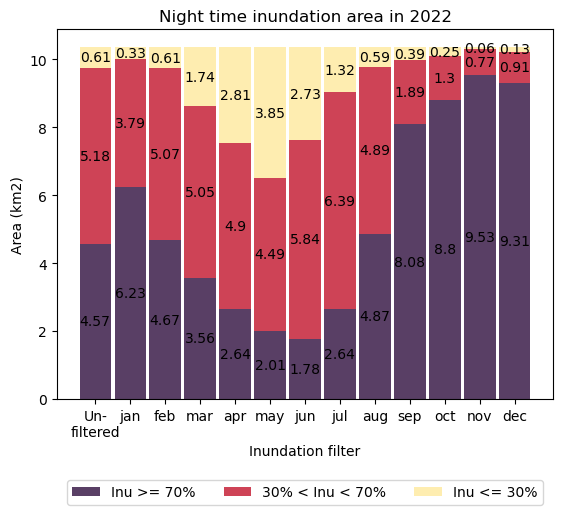
Interpretation
There is a strong pattern in the monthly night-time inundation characteristics of this location. Between September and January each year, more than half of the intertidal zone is inundated for more than 70 % of night-time hours.
This seasonality may be influential on relatively poorly understood dugong distributions and life-cycles. The nutritional content of intertidal seagrass varies with elevation and dugong have been observed to venture inshore at night to forage on varieties only available at high tide (e.g. Sheppard et al., 2010, Derville et al., 2022). There is some evidence that dugong herds are larger and less dispersed during spring and summer, when seagrass meadows are large and highly productive (Lanyon 2003). This analysis shows that those meadows are also readily accessible during preferred foraging hours at this time of the year. Female dugong fertility is correspondingly most active between July and December with calving concentrated around similar months (Marsh et al., 1984; Burgess., 2012), when nutritious food is abundant and accessible. Spatial and temporal mapping of exposure characteristics in known dugong habitat reveals that access to nutritious food, in addition to seagrass abundance, is linked to seasonality and may influence the life cycle and reproductive success of the vulnerable dugong species.
Mapping the exposure characteristics of intertidal habitats reveals important insights and influences on the distribution and life-cycles of the species that occupy them. Exposure time is a critically influential element in intertidal ecosystems and the ability to map it over time and space enables improved understanding of these environments for conservation and management.
Reference list
Buckee, J., Hetzel, Y., Edge, W., Verduin, J., & Pattiaratchi, C. (2022). Daily timing of low tide drives seasonality in intertidal emersion mortality risk. Frontiers in Marine Science, 9. https://doi.org/10.3389/fmars.2022.904191
Burgess, E. A. (2012). Determination of critical reproductive parameters of live, wild dugongs in a subtropical environment. https://espace.library.uq.edu.au/view/UQ:301919
Derville, S., Cleguer, C., & Garrigue, C. (2022). Ecoregional and temporal dynamics of dugong habitat use in a complex coral reef lagoon ecosystem. Scientific Reports, 12(1), 552. https://doi.org/10.1038/s41598-021-04412-3
Lanyon, J. (2003). Distribution and abundance of dugongs in Moreton Bay, Queensland, Australia. Wildl Res, 30. https://doi.org/10.1071/WR98082
Marsh, H., Heinsohn, G., & Marsh, L. (1984). Breeding Cycle, Life History and Population Dynamics of the Dugong, Dugon dugon (Sirenia: Dugongidae. Australian Journal of Zoology - AUST J ZOOL, 32. https://doi.org/10.1071/ZO9840767
Petrou, K., Jimenez-Denness, I., Chartrand, K., McCormack, C., Rasheed, M., & Ralph, P. (2013). Seasonal heterogeneity in the photophysiological response to air exposure in two tropical intertidal seagrass species. Marine Ecology Progress Series, 482, 93–106. https://doi.org/10.3354/meps10229
Sheppard, J. K., Marsh, H., Jones, R. E., & Lawler, I. R. (2010). Dugong habitat use in relation to seagrass nutrients, tides, and diel cycles. Marine Mammal Science, 26(4), 4. https://doi.org/10.1111/j.1748-7692.2010.00374.x
Yu, Y. Q., Zhang, Q. S., Tang, Y. Z., Li, X. M., Liu, H. L., & Li, L. X. (2013). Diurnal changes of photosynthetic quantum yield in the intertidal macroalga Sargassum thunbergii under simulated tidal emersion conditions. Journal of Sea Research, 80, 50–57. https://doi.org/10.1016/j.seares.2013.02.008
Additional information
License: The code in this notebook is licensed under the Apache License, Version 2.0. Digital Earth Australia data is licensed under the Creative Commons by Attribution 4.0 license.
Contact: If you need assistance, please post a question on the Open Data Cube Discord channel or on the GIS Stack Exchange using the open-data-cube tag (you can view previously asked questions here). If you would like to report an issue with this notebook, you can file one on
Github.
Last modified: February 2025
Compatible datacube version:
[13]:
print(datacube.__version__)
1.8.19
Tags
Browse all available tags on the DEA User Guide’s Tags Index
Tags: sandbox compatible, sentinel 2, landsat 8, rgb, DEA Intertidal, time series, GeoMAD, landsat 9