DEA Geometric Median and Median Absolute Deviation (Landsat)
DEA Geometric Median and Median Absolute Deviation (Landsat)
ga_ls5t_gm_cyear_3, ga_ls7e_gm_cyear_3, ga_ls8cls9c_gm_cyear_3
- Version:
- Type:
Derivative, Raster
- Resolution:
30 m
- Coverage:
1986 to 2025
- Data updates:
Yearly frequency, Ongoing
About
The DEA Geometric Median and Median Absolute Deviation products use statistical analyses to provide information on variance in the landscape over the given year. They provide insight into the “average” conditions observed over Australia in a given year, as well as the amount of variability experienced around that average. These products are useful for monitoring change detection, such as from cropping, urban expansion, or burnt area mapping.
This version includes breaking changes
All tile grid references have been changed to refer to a new origin point. Learn more in the Version 4.0.0 changelog.
Access the data
For help accessing the data, see the Access tab.
Key specifications
For more specifications, see the Specifications tab.
Technical name |
Geoscience Australia Landsat Geometric Median and Median Absolute Deviation Collection 3 |
Bands |
|
DOI |
|
Currency |
|
Parent product |
|
Collection |
|
Licence |
Cite this product
Data citation |
Geoscience Australia, 2022. DEA Geometric Median and Median Absolute Deviation (Landsat). Geoscience Australia, Canberra. https://dx.doi.org/10.26186/146261
|
Paper citation: Geometric Median |
Roberts, D., Mueller, N., Mcintyre, A., 2017. High-dimensional pixel composites from earth observation time series. IEEE Transactions on Geoscience and Remote Sensing, 55(11), 6254–6264. https://doi.org/10.1109/TGRS.2017.2723896
|
Paper citation: Median Absolute Deviation |
Roberts, D., Dunn, B., Mueller, N., 2018. Open data cube products using high-dimensional statistics of time series. IGARSS 2018 - 2018 IEEE International Geoscience and Remote Sensing Symposium, 8647–8650. https://doi.org/10.1109/IGARSS.2018.8518312
|
Publications
Roberts, D., Mueller, N., & Mcintyre, A. (2017). High-dimensional pixel composites from earth observation time series. IEEE Transactions on Geoscience and Remote Sensing, 55(11), 6254–6264. https://doi.org/10.1109/TGRS.2017.2723896
Roberts, D., Dunn, B., & Mueller, N. (2018). Open data cube products using high-dimensional statistics of time series. IGARSS 2018 - 2018 IEEE International Geoscience and Remote Sensing Symposium, 8647–8650. https://doi.org/10.1109/IGARSS.2018.8518312
Background
Satellite imagery allows us to observe the Earth with significant accuracy and detail. However, missing data — such as gaps caused by cloud cover — can make it difficult to create a complete image. In order to produce a single, complete view of a certain area, satellite data must be consolidated by stacking measurements from different points in time to create a composite image.
Large-scale image composites are increasingly important for a variety of applications such as land cover mapping, change detection, and the generation of high-quality data to parameterise and validate bio-physical and geophysical models. A number of compositing methodologies are being used in remote sensing in general, however challenges still exist. These challenges include mitigating against boundary artifacts due to mosaicking scenes from different epochs ensuring spatial regularity across the mosaic image and maintaining the spectral relationship between bands.
The creation of good composite images is especially important due to the opening of the Landsat archive of the United States Geological Survey. The greater availability of satellite imagery has resulted in demand to provide large regional mosaics that are representative of conditions over specific time periods while also being free of clouds and other unwanted visual noise. One approach is to ‘stitch together’ multiple selected high-quality images. Another is to create mosaics in which pixels from a time series of observations are combined (using an algorithm). This ‘pixel composite’ approach to mosaic generation provides more consistent results than with stitching high-quality images due to the improved colour balance created by combining one-by-one pixel-representative images. Another strength of pixel-based composites is their ability to be automated, hence enabling their use in large data collections and time series datasets.
The DEA GeoMAD product can be used for seeing how an area of land usually looks rather than only viewing it at a single point in time. Hence you can assess the land cover and land use on a general basis rather than at a specific date. It can also be used to assess how much an area changes over time. It highlights areas like bare rock that are very stable in contrast to cropping areas that change dramatically.
This product combines the Geometric Median and the Median Absolute Deviation algorithms in a single package. The Geometric Median output provides information on the general conditions of the landscape for a given year. Meanwhile the Median Absolute Deviation output provides information on how the landscape is changing in the same year.
What this product offers
This product provides statistical tools that utilise DEA’s Earth observation data to provide annual images of general conditions and how much an area changes in a given year.
The geometric median part of the product provides an ‘average’ cloud-free image over the given year. The geometric median image is calculated with a multi-dimensional median, using all the spectral measurements from the satellite imagery at the same time in order to maintain the relationships between the measurements.
The median absolute deviation part of the product uses three measures of variance, each of which provides a ‘second order’ high dimensional statistical composite for the given year. The three variance measures show how much an area varies from the ‘average’ in terms of ‘distance’ based on factors such as brightness and spectra. The three variance measures are: Euclidean distance (EMAD), Cosine (spectral) distance (SMAD), Bray Curtis dissimilarity (BCMAD).
They provide information on variance in the landscape over the given year and are useful for change detection applications.
The GeoMAD product is useful for the following:
Land cover mapping.
Change detection and classification (such as for burn-area mapping, crop mapping, and urban area mapping).
General variance and change, so it can be used in machine learning for change detection.
Environmental monitoring.
Technical information
Median Composites
Median composites are a method for creating large image mosaics using an algorithm that helps remove cloud and shadow noise by setting the value of each pixel of the composite to its consistent median values for each band. In this simple median method, the median of each band is independent of the other bands for any given pixel.
The benefit of using the median composite algorithm is that it is very fast to compute. The problem, however, is that satellite imagery pixels hold information for multiple bands and simple medians lose the relationships in this information, creating unnatural results. Therefore, a geometric median algorithm is used instead, since it can handle multi-dimensional data and maintain the relationships between bands for each pixel.
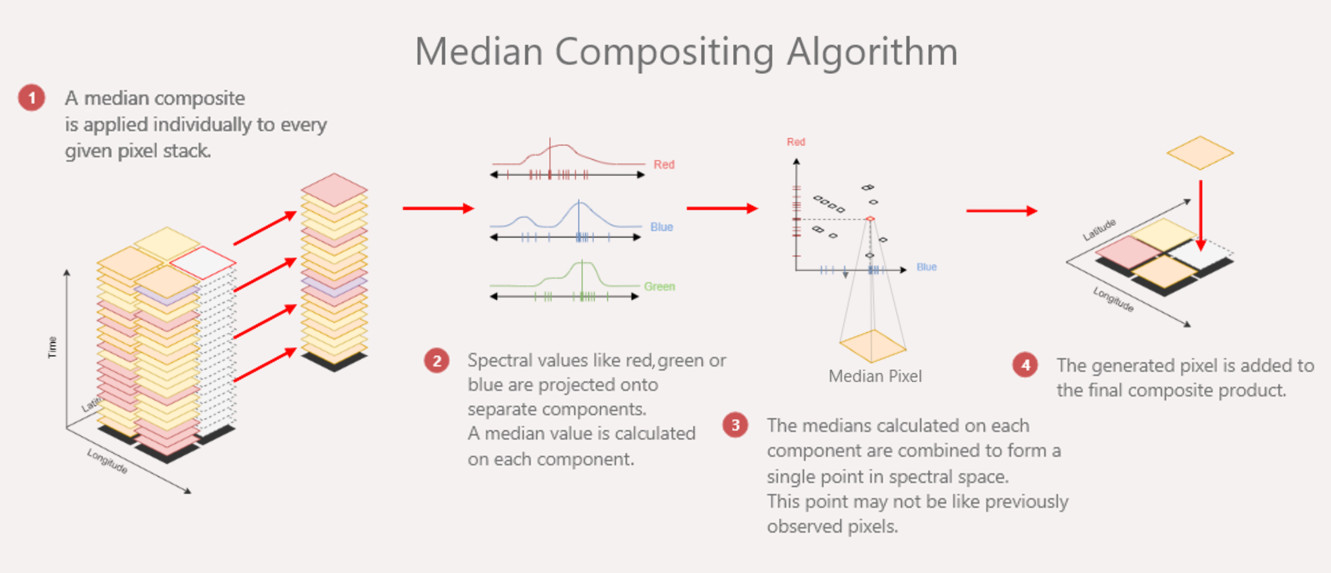
A simple median considers data from each band independently. This can be seen in Step 2 of the median compositing algorithm. (Source: Digital Earth Africa — Introduction to the Digital Earth Africa Sandbox)
Median Compositing Algorithm
As shown in the figure above, this algorithm is calculated as follows.
A median composite is applied individually to every given pixel stack
Spectral values like red, green, or blue are projected onto separate components. A median value is calculated on each component.
The medians calculated on each component are combined to form a single point in spectral space. This point may not be like previously observed pixels.
The generated pixel is added to the final composite product.
Geometric Median
Geometric Median composites are multi-band generalisations of median composites. A geometric median composite finds the median values of the bands for each pixel when considered together (as opposed to simple median composites which find a pixel’s median value for each band individually).
Geometric Medians are an appropriate choice of algorithm because they represent multiple bands of data.
The surface reflectance geometric median uses high-dimensional statistical theory to deliver a spectrally consistent and reasonably artefact-free pixel composite product.
The geometric median is a pixel-composite mosaic of a time series of earth observations. Essentially, the value of a pixel in a geometric median image is the statistical median of all observations for that pixel for a period of time. For example, the 2016 Landsat 8 geometric median image over an area will be the median of all Landsat 8 pixels recorded for that area in 2016.
An annual geometric median is a high-dimensional median calculated from the reflectance values recorded over a one-year period. The annual geometric median is available for each full calendar year since 1986.
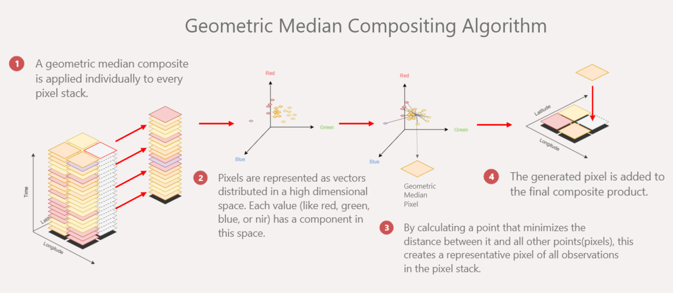
Each band adds a dimension to the geometric median calculation. For a three-band dataset — such as the RGB dataset shown in this figure — each point can be represented on a three-dimensional scatter plot. The geometric median is the minimised ‘sum of distances’ between all of these points. (Source: Digital Earth Africa — Introduction to the Digital Earth Africa Sandbox)
Geometric Median Compositing Algorithm
As shown in the figure above, this algorithm is calculated as follows.
A geometric median composite is applied individually to every pixel stack.
Pixels are represented as vectors distributed in a high-dimensional space. Each value (like red, green, blue, or NIR) has a component in this space. (NIR means Near-Infra Red.)
By calculating a point that minimises the distance between it and all other points (pixels), this creates a representative pixel of all observations in the pixel stack.
The generated pixel is added to the final composite product.
Multispectral satellite imagery (such as that provided by Landsat and Sentinel-2) consists of multiple measurements per pixel — one for each spectral band. In order to create a meaningful median, a median pixel must take all concurrent spectral measurements into account simultaneously as a multi-dimensional set (rather than each measurement independently as with a simple median). The geometric median is a high-dimensional statistic which calculates a multi-dimensional median from all the spectral measurements of the satellite imagery at the same time and maintains the relationships between the measurements. This provides a median of the physical conditions measured by the earth observations used to create it. It provides a good representation of a typical pixel observation devoid of outliers and has reduced spatial noise.
The annual geometric median provides an annual surface reflectance composite for any area of interest within the area covered by the DEA’s Open Data Cube, up to the entire spatial extent available. It provides a cloud-free overview of the middle surface reflectance value for each year. It is equivariant, meaning that a linear algorithm applied to a geometric median image is equal to a geometric median applied to a set of images on which the same linear algorithm was applied. Therefore, it can be used in further analyses such as Tasseled Cap, Principal Components Analysis, and Normalised Difference Indices. It is useful in analyses requiring baseline conditions such as change detection.
Surface reflectance geometric median products are derived from the DEA Surface Reflectance (SR) products and provide a representation of the ‘average’ of surface reflectance over the time period. This is a synthetic representation of a time series rather than an actual observed pixel.
The geometric median (Roberts et al. 2017) is used rather than the mean because the mean can be easily distorted by extrema whereas the median is less sensitive to outliers. The geometric median is used rather than the basic median because it preserves the physical relationship between spectral measurements. The geometric median is used rather than the medoid (Flood 2013) because a low noise composite cannot be provided. Note that where the provenance of each pixel in a composite is required, the medoid is the preferred method and the geometric median should not be used.
Input Data
The input data used to calculate the geometric median are filtered to remove poor quality observations. The filter only accepts observations with a geometric quality assessment (GQA) of less than 1 and it applies a 3-pixel opening operation on clouds and a 6-pixel dilation operation on both cloud and shadows for pixels masked by the fmask algorithm.
The statistics are calculated over time periods based on the availability of the satellites and sensors.
ga_ls5t_gm_cyear_3 — Uses Landsat 5 data.
ga_ls7e_gm_cyear_3 — Uses Landsat 7 data.
ga_ls8cls9c_gm_cyear_3 — Uses Landsat 8 and 9 data.
Note that only Landsat 7 geometric median data is available between 2000 and 2002 because the Landsat 5 satellite was unavailable.
The primary uses of geometric median pixel composites are for change detection within baselines and for broad regional image composites (such as national and continental mosaics).
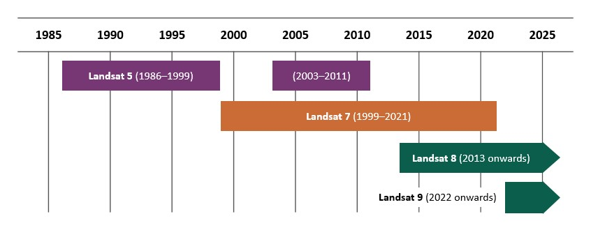
Timeline of Landsat satellite and sensor availability.
Timeline of Landsat availability
As shown in the figure above, the Landsat satellites have data available for the following time periods.
Landsat 5 |
1986–1999 and 2003–2011 |
Landsat 7 |
1999–2021 |
Landsat 8 |
2013 onwards |
Landsat 9 |
2022 onwards |
Median Absolute Deviation
The ‘first order’ statistics of a dataset include the mean and the median. As opposed to the mean, for multi-dimensional datasets such as satellite imagery, the median provides a method to find general conditions for a time period while also maintaining the physical relationships between spectral measurements.
A ‘second order’ statistic associated with a mean of a dataset is the standard deviation which provides a measure of data variance. The equivalent second order statistic associated with the median is the Median Absolute Deviation (MAD), which provides the associated variance measures for the median.
The MAD is the median of absolute differences of the individual values in a set of data from their overall median. To calculate the MAD for a multi-dimensional dataset — such as the set of satellite images captured in a year — measures of ‘distance’ from each multi-dimensional measurement to the median are needed. These are the set of spectral measurements for a pixel through time: blue, green, red, near-infra-red, and short-wave-infra-red. However, multi-dimensional distances can be calculated in different ways, providing different insights into the behaviour of pixels through time. The DEA GeoMAD product includes three MADs produced from different measures of distance.
Euclidean distance (EMAD) — this is more sensitive to changes in target brightness.
Cosine (spectral) distance (SMAD) — this is more sensitive to changes in target spectral response.
Bray Curtis dissimilarity (BCMAD) — this is more sensitive to the distribution of the observation values through time.
Each MAD provides information on different land cover change features; this is useful for classification.
The mathematical derivation of the three MADs can be found in Roberts et al. (2018).
More technical information …
Euclidean MAD (EMAD)
The most logical place to start thinking about any of the MADs is the Euclidean MAD (EMAD). This is because EMAD comes from Euclidean distance, and Euclidean distance can be explained with a physical analogy: it is how we measure straight-line distances between points. In our three-dimensional world, it may look like this:
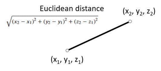
Euclidean distance in three dimensions.
In the case of satellite data, we are measuring the Euclidean distance between a pixel’s geometric median value and a single multispectral measurement. The number of dimensions is equal to the number of bands in the data. In the illustration below, \(m\) is the geometric median value and \(\mathbf{x}\) the measured value. In real data, there will be multiple measurements over a time period, so \(t\) is the timestep number, otherwise noted in equations as superscript (\(t\)).
For example, if we had three bands of data (red, green, and blue), and three timesteps of data, then we can calculate the Euclidean distances as follows:
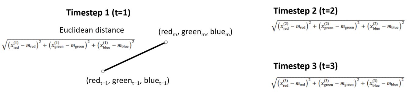
Euclidean distance in three dimensions over three timesteps.
Each timestep gives a separate Euclidean distance result. Then EMAD is the median of all those distances.
In most real life conditions, there will be more than three timesteps and more than three bands. A general expression of Euclidean distance for \(p\) bands is given as:
Then EMAD for \(N\) timesteps is given by Roberts et al, 2018, as the median of the Euclidean distances from all the timesteps.
In GeoMAD, the MADs are calculated from the same six bands used in the geometric median, therefore \(p=6\). The result of \(\lVert \mathbf{x}^{(t)} - \mathbf{m} \rVert_{\mathbb{R}^p}\) is a positive scalar, so \(\text{EMAD}_\text{GeoMAD}\) is a positive scalar number. As in the geometric median, \(N\) is dependent on the number of satellite flyovers particular to that pixel.
The maximum possible value for EMAD depends on the value ranges for each of the bands in the dataset. In the case of GeoMAD, which uses at maximum annual timescales of six bands of Landsat data, valid EMAD values range from 0 to 10000.
EMAD is useful for showing albedo shifts in satellite spectra.
(Source: Digital Earth Africa — GeoMAD cloud-free composites)
Spectral MAD (SMAD)
The spectral MAD (SMAD) is based on the median absolute deviations in the cosine distance between the geometric median and individual measurements.
In two dimensions, cosine distance can be graphically compared to Euclidean distance by the following figure:
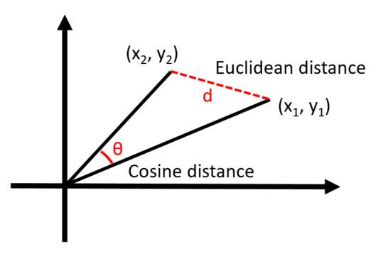
Relative relationships between Euclidean and cosine distances.
In a general sense, cosine distance is related to the angle between the two points \(\theta\), while Euclidean distance is related to the straight-line distance between the two points \(d\). Like Euclidean distance, points are more similar when the cosine distance between them is small. The value of the cosine distance is smaller when \(\theta\) is small (i.e. close to 0) or when \(\theta\) is close to 180 degrees.
Notice we could have a small cosine distance but a large Euclidean distance; for example, if the angle between the vectors is small, but one is much longer than the other. This is an important property of cosine distance (and thus SMAD) — unlike Euclidean distance, cosine distance is not skewed by the magnitude of the measurements.
Cosine distance is defined more formally as:
For more than two dimensions, we can generalise the cosine distance formula for a single pixel. For a multispectral measurement of \(p\) bands at timestep \(t\), \(\mathbf{x}^{(t)}\), and the geometric median at the same point \(\mathbf{m}\), the cosine distance is:
Then for \(N\) timesteps, SMAD is the median of the cosine distances.
As with the other distances and dissimilarities used in the MADs, this results in a positive scalar value, thus SMAD is a positive scalar. Valid values for SMAD fall between 0 and 1.
In applications of Earth observation data, SMAD is useful for showing areas of land cover change. One reason is that SMAD is less affected by cloud; unlike EMAD, it is invariant to albedo changes, such as that caused by the diffusion of solar radiation. SMAD can also be used to track water bodies, as water has high variation in reflectance.
(Source: Digital Earth Africa — GeoMAD cloud-free composites)
Bray-Curtis MAD (BCMAD)
The Bray-Curtis MAD (BCMAD) is calculated from the Bray-Curtis dissimilarity. The Bray-Curtis dissimilarity emphasises differences in each band between the measurement and the geometric median.
For a single band of satellite data, the Bray-Curtis dissimilarity looks remarkably like a normalised band index. For example, if we only had red band data, it might look something like this:
It can be generalised to a multispectral dataset with \(p\) bands:
The Bray-Curtis dissimilarity will be maximised at a value of 1 when the measurements in each band are completely different. Conversely, the value of the dissimilarity will be small where each band observation is similar to the geometric median of that band.
As with the other MADs, the BCMAD is found by taking the median of all the Bray-Curtis dissimilarities from \(N\) timesteps. For GeoMAD, \(p=10\).
BCMAD takes on values from 0 to 1.
(Source: Digital Earth Africa — GeoMAD cloud-free composites)
Lineage

Landsat 5, 7, 8, and 9 Surface Reflectance includes NBART and Observational Attributes products. GeoMAD stands for Geometric Median and Median Absolute Deviation.
The GeoMAD is derived from Landsat surface reflectance data. The data are masked for clouds and shadows to increase clarity and ensure the best data is used in the median calculation.
The three MAD layers of the GeoMAD are calculated by computing the multidimensional distance between each observation in a time series of multispectral (or higher dimensionality such as hyperspectral) satellite imagery versus the multidimensional median of the time series. The median used for this calculation is the geometric median corresponding to the time series.
The GeoMAD is calculated over annual time periods on Earth observations from a single sensor by default (such as the annual time series of Landsat 8 observations); however it is applicable to multi-sensor time series of any length that computing resources can support.
For the purposes of the default DEA product, GeoMADs are computed per calendar year per sensor for Landsat 5, Landsat 7, and Landsat 8 until 2021. GeoMADs are computed from combined sensors Landsat 8 and Landsat 9 from 2022 onwards. GeoMADs are computed using terrain-illumination-corrected surface reflectance data (Analysis Ready Data).
Note that the constituent pixels in the GeoMAD pixel composite mosaics are synthetic. This means that the pixels have not been physically observed by the satellite; rather, they are the computed high-dimensional medians of a time series of pixels.
References
Roberts, D., Mueller, N., & Mcintyre, A. (2017). High-dimensional pixel composites from earth observation time series. IEEE Transactions on Geoscience and Remote Sensing, 55(11), 6254–6264. https://doi.org/10.1109/TGRS.2017.2723896
Roberts, D., Dunn, B., & Mueller, N. (2018). Open data cube products using high-dimensional statistics of time series. IGARSS 2018 - 2018 IEEE International Geoscience and Remote Sensing Symposium, 8647–8650. https://doi.org/10.1109/IGARSS.2018.8518312
Accuracy
The accuracy of the GeoMAD layers is dependent on the accuracy of the earth observation data on which it is based.
To calculate a reliable geometric median or MAD, the majority of the input data must be free of clouds, shadows, or other visual obstructions. For locations that experience more than 50% of time under clouds and shadows (such as areas of Tasmania) the GeoMAD can produce an output that is obscured by visual noise. Therefore, it is necessary to use a large enough collection of data to prevent this occurring.
To reduce the impact of poor-quality earth observation data, the input data is screened using the Pixel Quality product.
Note that where no-data pixels occur in locations that clear observations should occur, the cause is a lack of clear pixels to populate the GeoMAD.
Also, note that since the geometric median and MAD are synthetic (not observed directly by satellite), they cannot be verified by field work.
Product IDs
The Product IDs are ga_ls5t_gm_cyear_3, ga_ls7e_gm_cyear_3, and ga_ls8cls9c_gm_cyear_3. These IDs are used to load data from the Open Data Cube (ODC), for example dc.load(product="ga_ls5t_gm_cyear_3", ...)
Bands
Bands are distinct layers of data within a product that can be loaded using the Open Data Cube (on the DEA Sandbox or NCI) or DEA’s STAC API. Note that the Coordinate Reference System (CRS) of these bands is GDA94 / Australian Albers (EPSG:3577).
Type |
Units |
Resolution |
No-data |
Aliases |
Description |
|
|---|---|---|---|---|---|---|
nbart_blue |
int16 |
- |
30 m |
-999 |
- |
- |
nbart_green |
int16 |
- |
30 m |
-999 |
- |
- |
nbart_red |
int16 |
- |
30 m |
-999 |
- |
- |
nbart_nir |
int16 |
- |
30 m |
-999 |
- |
- |
nbart_swir_1 |
int16 |
- |
30 m |
-999 |
- |
- |
nbart_swir_2 |
int16 |
- |
30 m |
-999 |
- |
- |
sdev |
float32 |
- |
30 m |
NaN |
- |
- |
edev |
float32 |
- |
30 m |
NaN |
- |
- |
bcdev |
float32 |
- |
30 m |
NaN |
- |
- |
count |
int16 |
- |
30 m |
-999 |
- |
- |
For all ‘nbart_’ bands, Surface Reflectance is scaled between 0 and 10,000.
Product information
This metadata provides general information about the product.
Product IDs |
ga_ls5t_gm_cyear_3
ga_ls7e_gm_cyear_3
ga_ls8cls9c_gm_cyear_3
|
Used to load data from the Open Data Cube. |
Short name |
DEA Geometric Median and Median Absolute Deviation (Landsat) |
The name that is commonly used to refer to the product. |
Technical name |
Geoscience Australia Landsat Geometric Median and Median Absolute Deviation Collection 3 |
The full technical name that refers to the product and its specific provider, sensors, and collection. |
Version |
4.0.0 |
The version number of the product. See the History tab. |
Lineage type |
Derivative |
Derivative products are derived from other products. |
Spatial type |
Raster |
Raster data consists of a grid of pixels. |
Spatial resolution |
30 m |
The size of the pixels in the raster. |
Temporal coverage |
1986 to 2025 |
The time span for which data is available. |
Coordinate Reference System (CRS) |
The method of mapping spatial data to the Earth’s surface. |
|
Update frequency |
Yearly |
The expected frequency of data updates. Also called ‘Temporal resolution’. |
Update activity |
Ongoing |
The activity status of data updates. |
Currency |
Currency is a measure based on data publishing and update frequency. |
|
Latest and next update dates |
See Table B of the report. |
|
DOI |
The Digital Object Identifier. |
|
Catalogue ID |
The Data and Publications catalogue (eCat) ID. |
|
Licence |
See the Credits tab. |
Product categorisation
This metadata describes how the product relates to other products.
Parent product |
|
Collection |
|
Tags |
geoscience_australia_landsat_collection_3, satellite_images, geomedian, geo_mad, geometric_median, median_absolute_deviation |
Access the data
DEA Maps |
Learn how to use DEA Maps. |
|
DEA Explorer |
Learn how to use the DEA Explorer. |
|
Data sources |
Learn how to access the data via AWS. |
|
Code examples |
Learn how to use the DEA Sandbox. |
|
Web services |
Learn how to use DEA’s web services. |
Accessing the web services
When accessing the product via the OGC Web Services, the layer names for the data are ga_ls5t_gm_cyear_3, ga_ls7e_gm_cyear_3, and ga_ls8cls9c_gm_cyear_3. Learn about these layers on the Details tab.
Version history
Versions are numbered using the Semantic Versioning scheme (Major.Minor.Patch). Note that this list may include name changes and predecessor products.
v4.0.0 |
- |
Current version |
v3.1.0 |
of |
DEA Geometric Median and Median Absolute Deviation (Landsat) |
v2.1.0 |
of |
|
v2.0.0 |
of |
Changelog
30 Apr 2026: 2025 annual update now available
Digital Earth Australia (DEA) delivers refreshed 2025 annual data for a suite of terrestrial and inland water products, ensuring they reflect the most recent full calendar year of observations and remain consistent across the DEA product catalogue.
These updated datasets support consistent, year‑to‑year analysis of Australia’s land and inland water environments, helping users monitor change, compare trends over time, and apply the latest information with confidence.
By refreshing these products on an annual cycle, DEA continues to provide a nationally consistent foundation for land and water analysis, aligned across the broader DEA product catalogue.
16 Feb 2026: Issue notification removed
A potential issue was identified in September 2024 affecting the DEA Geometric Median and Median Absolute Deviation (Landsat) product. A bug in the processing code related to multithreading with numexpr may have caused a 400 × 400 pixel data block to be misplaced (effectively, duplicated) within a small number of tiles.
Initial estimates suggested that approximately 8–12 tiles across the full GeoMAD archive could have been affected; however, the specific tiles were unknown.
The underlying cause was subsequently identified and fixed in the codebase.
In late 2025, the entire GeoMAD data repository was programmatically reviewed to detect any duplicated 400 × 400 pixel data blocks within each tile, excluding blocks that were fully no‑data. No evidence of affected tiles was found.
Based on this investigation, the issue is now considered resolved, and the notification has been moved to the change log.
30 Apr 2025: The 2024 annual data is now available
You are now able to access the latest data via DEA Maps and other methods. View the Tech Alert.
Version 4.0.0
Breaking change: Shift in grid origin point — The south-west origin point of the DEA Summary Product Grid has been shifted 18 tiles west and 15 tiles south. Therefore, all tile grid references have been changed. For instance, a tile reference of
x10y10has changed tox28y25. The tile grid references of all derivative products generated from 2024 onwards will also be changed; however, Analysis Ready Data products will not be affected.Enhanced cloud masking to reduce noise — An enhancement to cloud masking has reduced cloud and shadow noise. This enhancement (known as ‘cloud buffering’) involved cleaning cloud masks using a 3-pixel morphological opening on clouds and a 6-pixel dilation on cloud and shadows. Note that some areas of very high surface reflectance (e.g. sand dunes and ocean areas) may exhibit worsened noise or data gaps, but these are infrequent occurrences with low impact.
Combined Landsat 8 and 9 product — A single combined product for Landsat 8 and Landsat 9 is provided. It achieves better performance than the standalone Landsat 8 product due to using a larger number of available observations. A standalone Landsat 8 product will no longer be provided from calendar year 2022 onwards.
Prefixed band measurement names — An ‘nbart’ prefix was added to band measurement names for consistency with our Analysis Ready Data products. For example, the
redband has been renamed tonbart_red.
Acknowledgments
The high-dimensional statistics algorithms incorporated in this product is the work of Dr Dale Roberts, Australian National University.
License and copyright
© Commonwealth of Australia (Geoscience Australia).
Released under Creative Commons Attribution 4.0 International Licence.