SpatioTemporal Asset Catalogue (STAC)
SpatioTemporal Asset Catalog (STAC) is a specification that consistently describes geospatial information so it can more easily be discovered and accessed. STAC provides a powerful tool to quickly identify all available data for a given product, location or time period. This data can then be easily and efficiently loaded into your own computing environment, or streamed directly into desktop GIS software like QGIS or ESRI.
Why use STAC?
STAC may be useful for you if any of the following apply:
You want to easily find and load satellite data products through time or across large spatial areas
You want to access satellite data on your own computing environment
Your analysis requires more memory or processing power than provided by DEA’s managed Sandbox or NCI environments
You want to combine DEA data with data from other external sources (e.g. Microsoft Planetary Computer, Element 84 Earth Search)
odc-stac tutorial
This tutorial demonstrates how to use the odc-stac Python package to load data from DEA using the DEA Explorer STAC API. The odc-stac package translates STAC metadata to the Open Data Cube data model (Table 1), allowing you to load DEA data into xarray.Dataset format to be processed locally, or distribute data loading and computation with
Dask.
Table 1: Comparison between STAC and Open Data Cube concepts
STAC |
ODC |
Description |
|---|---|---|
A collection of observations across space and time (e.g. all observations from a Landsat or Sentinel-2 satellite sensor) |
||
A single observation for a specific time and place, containing one or more bands (for example, a specific Landsat or Sentinel-2 scene) |
||
A component of an observation, including but not limited to bands |
||
A single data layer/array within a multi-band observation (e.g. spectral data from a specific wavelength) |
||
Alias |
Alternative names for the same band |
Setup
Import required packages for querying and loading data from STAC:
[1]:
import pystac_client
import odc.stac
Connect to the DEA Explorer STAC API to allow searching for data:
[2]:
catalog = pystac_client.Client.open("https://explorer.dea.ga.gov.au/stac")
To load data via STAC, we must configure appropriate access to data stored on DEA’s Amazon S3 buckets. This can be done with the odc.stac.configure_rio function. The configuration below must be used when loading any DEA data through the STAC API.
[3]:
odc.stac.configure_rio(
    cloud_defaults=True,
    aws={"aws_unsigned": True},
)
Searching for STAC data using pystac_client
First we need to define the location, time period and DEA product we want to load.
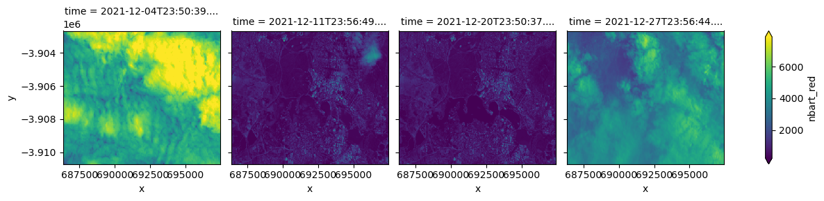
In this example, we will load December 2021 Landsat 8 data over Canberra:
[4]:
# Set a bounding box
# [xmin, ymin, xmax, ymax] in latitude and longitude
bbox = [149.05, -35.32, 149.17, -35.25]

# Set a start and end date
start_date = "2021-12-01"
end_date = "2021-12-31"

# Set product ID as the STAC "collection"
collections = ["ga_ls8c_ard_3"]
Now we can use the pystac_client Python package to search for STAC items that match our query:
[5]:
# Build a query with the parameters above
query = catalog.search(
    bbox=bbox,
    collections=collections,
    datetime=f"{start_date}/{end_date}",
)

# Search the STAC catalog for all items matching the query
items = list(query.items())
print(f"Found: {len(items):d} datasets")
Found: 8 datasets
Loading data using odc-stac
Once we have found data to load, we can use the odc.stac.load() function to load them as xarray.Dataset format.
This works similarly to how the datacube.load() function is used to load data from DEA on the DEA Sandbox and on the NCI.
[6]:
ds = odc.stac.load(
    items,
    bands=["nbart_red"],
    crs="utm",
    resolution=30,
    groupby="solar_day",
    bbox=bbox,
)

ds
[6]:
<xarray.Dataset> Size: 2MB
Dimensions:      (y: 268, x: 370, time: 4)
Coordinates:
  * y            (y) float64 2kB -3.903e+06 -3.903e+06 ... -3.911e+06 -3.911e+06
  * x            (x) float64 3kB 6.864e+05 6.864e+05 ... 6.974e+05 6.974e+05
    spatial_ref  int32 4B 32655
  * time         (time) datetime64[ns] 32B 2021-12-04T23:50:39.744022 ... 202...
Data variables:
nbart_red (time, y, x) float32 2MB 5.597e+03 5.571e+03 ... 5.203e+03We can now plot and analyse our data:
[7]:
ds.nbart_red.plot(col="time", robust=True);
Advanced
Filtering
The DEA STAC API supports filtering data by metadata fields before loading it using the filter extention parameter. This can be useful for limiting data loads to the most useful data (e.g. least affected by clouds, most geometrically accurate etc).
To inspect the fields we can filter on, we can look at a single STAC item and expand the properties dropdown:
[8]:
items[0]
[8]:
- type "Feature"
- stac_version "1.0.0"
- id "fa4b50d5-22ee-4fc3-ba72-ae306696778a"
properties
- title "ga_ls8c_ard_3-2-0_090084_2021-12-04_final"
- gsd 15.0
- created "2021-12-16T11:02:09.430131Z"
- gqa:abs_x "NaN"
- gqa:abs_y "NaN"
- gqa:cep90 "NaN"
- proj:epsg 32655
- fmask:snow 0.0
- gqa:abs_xy "NaN"
- gqa:mean_x "NaN"
- gqa:mean_y "NaN"
proj:shape[] 2 items
- 0 7951
- 1 7911
- platform "landsat-8"
- fmask:clear 12.899177700739955
- fmask:cloud 85.11645459806458
- fmask:water 0.10471018298970154
- gqa:mean_xy "NaN"
- odc:product "ga_ls8c_ard_3"
- gqa:stddev_x "NaN"
- gqa:stddev_y "NaN"
- odc:producer "ga.gov.au"
instruments[] 2 items
- 0 "oli"
- 1 "tirs"
- gqa:stddev_xy "NaN"
- eo:cloud_cover 85.11645459806458
- view:sun_azimuth 73.06249576
proj:transform[] 9 items
- 0 30.0
- 1 0.0
- 2 641985.0
- 3 0.0
- 4 -30.0
- 5 -3714585.0
- 6 0.0
- 7 0.0
- 8 1.0
- landsat:wrs_row 84
- odc:file_format "GeoTIFF"
- odc:region_code "090084"
- end_datetime "2021-12-04T23:50:54.297148Z"
- view:sun_elevation 60.99075226
- landsat:wrs_path 90
- start_datetime "2021-12-04T23:50:25.043607Z"
- fmask:cloud_shadow 1.8796575182057698
- odc:product_family "ard"
- odc:dataset_version "3.2.0"
- dea:dataset_maturity "final"
- gqa:iterative_mean_x "NaN"
- gqa:iterative_mean_y "NaN"
- gqa:iterative_mean_xy "NaN"
- gqa:iterative_stddev_x "NaN"
- gqa:iterative_stddev_y "NaN"
- gqa:iterative_stddev_xy "NaN"
- gqa:abs_iterative_mean_x "NaN"
- gqa:abs_iterative_mean_y "NaN"
- landsat:landsat_scene_id "LC80900842021338LGN00"
- gqa:abs_iterative_mean_xy "NaN"
- landsat:collection_number 1
- landsat:landsat_product_id "LC08_L1GT_090084_20211204_20211214_01_T2"
- landsat:collection_category "T2"
- cubedash:region_code "090084"
- datetime "2021-12-04T23:50:39.744022Z"
geometry
- type "Polygon"
coordinates[] 1 items
0[] 21 items
0[] 2 items
- 0 150.63644964806994
- 1 -35.666308392803934
1[] 2 items
- 0 150.63639206845306
- 1 -35.66649935644676
2[] 2 items
- 0 148.56660409360416
- 1 -35.26715358267796
3[] 2 items
- 0 148.56663480869796
- 1 -35.26703597804695
4[] 2 items
- 0 148.56607186822058
- 1 -35.26691704471369
5[] 2 items
- 0 148.5667898774827
- 1 -35.26367103415514
6[] 2 items
- 0 148.57483626542418
- 1 -35.236383544412845
7[] 2 items
- 0 148.64752850197317
- 1 -34.99117220990075
8[] 2 items
- 0 148.94947724153644
- 1 -33.96925067274828
9[] 2 items
- 0 149.05004319115557
- 1 -33.626232352212824
10[] 2 items
- 0 149.0709859121868
- 1 -33.55544079095941
11[] 2 items
- 0 149.07182585726682
- 1 -33.555435748897885
12[] 2 items
- 0 149.09033291555275
- 1 -33.559182270747755
13[] 2 items
- 0 149.65444990470453
- 1 -33.67200805540741
14[] 2 items
- 0 151.09939917481952
- 1 -33.9477017314025
15[] 2 items
- 0 151.09938017853193
- 1 -33.94775642659265
16[] 2 items
- 0 151.10025279065292
- 1 -33.94791653232726
17[] 2 items
- 0 151.10032794539072
- 1 -33.94858078379386
18[] 2 items
- 0 151.09072130580546
- 1 -33.98498710194393
19[] 2 items
- 0 150.63764094939643
- 1 -35.666524659346386
20[] 2 items
- 0 150.63644964806994
- 1 -35.666308392803934
links[] 7 items
0
- rel "self"
- href "https://explorer.dea.ga.gov.au/stac/collections/ga_ls8c_ard_3/items/fa4b50d5-22ee-4fc3-ba72-ae306696778a"
- type "application/json"
1
- rel "odc_yaml"
- href "https://explorer.dea.ga.gov.au/dataset/fa4b50d5-22ee-4fc3-ba72-ae306696778a.odc-metadata.yaml"
- type "text/yaml"
- title "ODC Dataset YAML"
2
- rel "collection"
- href "https://explorer.dea.ga.gov.au/stac/collections/ga_ls8c_ard_3"
3
- rel "product_overview"
- href "https://explorer.dea.ga.gov.au/product/ga_ls8c_ard_3"
- type "text/html"
- title "ODC Product Overview"
4
- rel "alternative"
- href "https://explorer.dea.ga.gov.au/dataset/fa4b50d5-22ee-4fc3-ba72-ae306696778a"
- type "text/html"
- title "ODC Dataset Overview"
5
- rel "canonical"
- href "https://data.dea.ga.gov.au/?prefix=baseline/ga_ls8c_ard_3/090/084/2021/12/04/"
- type "application/json"
6
- rel "root"
- href "https://explorer.dea.ga.gov.au/stac"
- type "application/json"
- title "AWS Explorer"
assets
oa_fmask
- href "s3://dea-public-data/baseline/ga_ls8c_ard_3/090/084/2021/12/04/ga_ls8c_oa_3-2-0_090084_2021-12-04_final_fmask.tif"
- type "image/tiff; application=geotiff; profile=cloud-optimized"
- title "oa_fmask"
eo:bands[] 1 items
0
- name "oa_fmask"
- proj:epsg 32655
proj:shape[] 2 items
- 0 7951
- 1 7911
proj:transform[] 9 items
- 0 30.0
- 1 0.0
- 2 641985.0
- 3 0.0
- 4 -30.0
- 5 -3714585.0
- 6 0.0
- 7 0.0
- 8 1.0
roles[] 1 items
- 0 "data"
nbart_nir
- href "s3://dea-public-data/baseline/ga_ls8c_ard_3/090/084/2021/12/04/ga_ls8c_nbart_3-2-0_090084_2021-12-04_final_band05.tif"
- type "image/tiff; application=geotiff; profile=cloud-optimized"
- title "nbart_nir"
eo:bands[] 1 items
0
- name "nbart_nir"
- proj:epsg 32655
proj:shape[] 2 items
- 0 7951
- 1 7911
proj:transform[] 9 items
- 0 30.0
- 1 0.0
- 2 641985.0
- 3 0.0
- 4 -30.0
- 5 -3714585.0
- 6 0.0
- 7 0.0
- 8 1.0
roles[] 1 items
- 0 "data"
nbart_red
- href "s3://dea-public-data/baseline/ga_ls8c_ard_3/090/084/2021/12/04/ga_ls8c_nbart_3-2-0_090084_2021-12-04_final_band04.tif"
- type "image/tiff; application=geotiff; profile=cloud-optimized"
- title "nbart_red"
eo:bands[] 1 items
0
- name "nbart_red"
- proj:epsg 32655
proj:shape[] 2 items
- 0 7951
- 1 7911
proj:transform[] 9 items
- 0 30.0
- 1 0.0
- 2 641985.0
- 3 0.0
- 4 -30.0
- 5 -3714585.0
- 6 0.0
- 7 0.0
- 8 1.0
roles[] 1 items
- 0 "data"
nbart_blue
- href "s3://dea-public-data/baseline/ga_ls8c_ard_3/090/084/2021/12/04/ga_ls8c_nbart_3-2-0_090084_2021-12-04_final_band02.tif"
- type "image/tiff; application=geotiff; profile=cloud-optimized"
- title "nbart_blue"
eo:bands[] 1 items
0
- name "nbart_blue"
- proj:epsg 32655
proj:shape[] 2 items
- 0 7951
- 1 7911
proj:transform[] 9 items
- 0 30.0
- 1 0.0
- 2 641985.0
- 3 0.0
- 4 -30.0
- 5 -3714585.0
- 6 0.0
- 7 0.0
- 8 1.0
roles[] 1 items
- 0 "data"
nbart_green
- href "s3://dea-public-data/baseline/ga_ls8c_ard_3/090/084/2021/12/04/ga_ls8c_nbart_3-2-0_090084_2021-12-04_final_band03.tif"
- type "image/tiff; application=geotiff; profile=cloud-optimized"
- title "nbart_green"
eo:bands[] 1 items
0
- name "nbart_green"
- proj:epsg 32655
proj:shape[] 2 items
- 0 7951
- 1 7911
proj:transform[] 9 items
- 0 30.0
- 1 0.0
- 2 641985.0
- 3 0.0
- 4 -30.0
- 5 -3714585.0
- 6 0.0
- 7 0.0
- 8 1.0
roles[] 1 items
- 0 "data"
nbart_swir_1
- href "s3://dea-public-data/baseline/ga_ls8c_ard_3/090/084/2021/12/04/ga_ls8c_nbart_3-2-0_090084_2021-12-04_final_band06.tif"
- type "image/tiff; application=geotiff; profile=cloud-optimized"
- title "nbart_swir_1"
eo:bands[] 1 items
0
- name "nbart_swir_1"
- proj:epsg 32655
proj:shape[] 2 items
- 0 7951
- 1 7911
proj:transform[] 9 items
- 0 30.0
- 1 0.0
- 2 641985.0
- 3 0.0
- 4 -30.0
- 5 -3714585.0
- 6 0.0
- 7 0.0
- 8 1.0
roles[] 1 items
- 0 "data"
nbart_swir_2
- href "s3://dea-public-data/baseline/ga_ls8c_ard_3/090/084/2021/12/04/ga_ls8c_nbart_3-2-0_090084_2021-12-04_final_band07.tif"
- type "image/tiff; application=geotiff; profile=cloud-optimized"
- title "nbart_swir_2"
eo:bands[] 1 items
0
- name "nbart_swir_2"
- proj:epsg 32655
proj:shape[] 2 items
- 0 7951
- 1 7911
proj:transform[] 9 items
- 0 30.0
- 1 0.0
- 2 641985.0
- 3 0.0
- 4 -30.0
- 5 -3714585.0
- 6 0.0
- 7 0.0
- 8 1.0
roles[] 1 items
- 0 "data"
oa_time_delta
- href "s3://dea-public-data/baseline/ga_ls8c_ard_3/090/084/2021/12/04/ga_ls8c_oa_3-2-0_090084_2021-12-04_final_time-delta.tif"
- type "image/tiff; application=geotiff; profile=cloud-optimized"
- title "oa_time_delta"
eo:bands[] 1 items
0
- name "oa_time_delta"
- proj:epsg 32655
proj:shape[] 2 items
- 0 7951
- 1 7911
proj:transform[] 9 items
- 0 30.0
- 1 0.0
- 2 641985.0
- 3 0.0
- 4 -30.0
- 5 -3714585.0
- 6 0.0
- 7 0.0
- 8 1.0
roles[] 1 items
- 0 "data"
oa_solar_zenith
- href "s3://dea-public-data/baseline/ga_ls8c_ard_3/090/084/2021/12/04/ga_ls8c_oa_3-2-0_090084_2021-12-04_final_solar-zenith.tif"
- type "image/tiff; application=geotiff; profile=cloud-optimized"
- title "oa_solar_zenith"
eo:bands[] 1 items
0
- name "oa_solar_zenith"
- proj:epsg 32655
proj:shape[] 2 items
- 0 7951
- 1 7911
proj:transform[] 9 items
- 0 30.0
- 1 0.0
- 2 641985.0
- 3 0.0
- 4 -30.0
- 5 -3714585.0
- 6 0.0
- 7 0.0
- 8 1.0
roles[] 1 items
- 0 "data"
oa_exiting_angle
- href "s3://dea-public-data/baseline/ga_ls8c_ard_3/090/084/2021/12/04/ga_ls8c_oa_3-2-0_090084_2021-12-04_final_exiting-angle.tif"
- type "image/tiff; application=geotiff; profile=cloud-optimized"
- title "oa_exiting_angle"
eo:bands[] 1 items
0
- name "oa_exiting_angle"
- proj:epsg 32655
proj:shape[] 2 items
- 0 7951
- 1 7911
proj:transform[] 9 items
- 0 30.0
- 1 0.0
- 2 641985.0
- 3 0.0
- 4 -30.0
- 5 -3714585.0
- 6 0.0
- 7 0.0
- 8 1.0
roles[] 1 items
- 0 "data"
oa_solar_azimuth
- href "s3://dea-public-data/baseline/ga_ls8c_ard_3/090/084/2021/12/04/ga_ls8c_oa_3-2-0_090084_2021-12-04_final_solar-azimuth.tif"
- type "image/tiff; application=geotiff; profile=cloud-optimized"
- title "oa_solar_azimuth"
eo:bands[] 1 items
0
- name "oa_solar_azimuth"
- proj:epsg 32655
proj:shape[] 2 items
- 0 7951
- 1 7911
proj:transform[] 9 items
- 0 30.0
- 1 0.0
- 2 641985.0
- 3 0.0
- 4 -30.0
- 5 -3714585.0
- 6 0.0
- 7 0.0
- 8 1.0
roles[] 1 items
- 0 "data"
oa_incident_angle
- href "s3://dea-public-data/baseline/ga_ls8c_ard_3/090/084/2021/12/04/ga_ls8c_oa_3-2-0_090084_2021-12-04_final_incident-angle.tif"
- type "image/tiff; application=geotiff; profile=cloud-optimized"
- title "oa_incident_angle"
eo:bands[] 1 items
0
- name "oa_incident_angle"
- proj:epsg 32655
proj:shape[] 2 items
- 0 7951
- 1 7911
proj:transform[] 9 items
- 0 30.0
- 1 0.0
- 2 641985.0
- 3 0.0
- 4 -30.0
- 5 -3714585.0
- 6 0.0
- 7 0.0
- 8 1.0
roles[] 1 items
- 0 "data"
oa_relative_slope
- href "s3://dea-public-data/baseline/ga_ls8c_ard_3/090/084/2021/12/04/ga_ls8c_oa_3-2-0_090084_2021-12-04_final_relative-slope.tif"
- type "image/tiff; application=geotiff; profile=cloud-optimized"
- title "oa_relative_slope"
eo:bands[] 1 items
0
- name "oa_relative_slope"
- proj:epsg 32655
proj:shape[] 2 items
- 0 7951
- 1 7911
proj:transform[] 9 items
- 0 30.0
- 1 0.0
- 2 641985.0
- 3 0.0
- 4 -30.0
- 5 -3714585.0
- 6 0.0
- 7 0.0
- 8 1.0
roles[] 1 items
- 0 "data"
oa_satellite_view
- href "s3://dea-public-data/baseline/ga_ls8c_ard_3/090/084/2021/12/04/ga_ls8c_oa_3-2-0_090084_2021-12-04_final_satellite-view.tif"
- type "image/tiff; application=geotiff; profile=cloud-optimized"
- title "oa_satellite_view"
eo:bands[] 1 items
0
- name "oa_satellite_view"
- proj:epsg 32655
proj:shape[] 2 items
- 0 7951
- 1 7911
proj:transform[] 9 items
- 0 30.0
- 1 0.0
- 2 641985.0
- 3 0.0
- 4 -30.0
- 5 -3714585.0
- 6 0.0
- 7 0.0
- 8 1.0
roles[] 1 items
- 0 "data"
nbart_panchromatic
- href "s3://dea-public-data/baseline/ga_ls8c_ard_3/090/084/2021/12/04/ga_ls8c_nbart_3-2-0_090084_2021-12-04_final_band08.tif"
- type "image/tiff; application=geotiff; profile=cloud-optimized"
- title "nbart_panchromatic"
eo:bands[] 1 items
0
- name "nbart_panchromatic"
- proj:epsg 32655
proj:shape[] 2 items
- 0 15901
- 1 15821
proj:transform[] 9 items
- 0 15.0
- 1 0.0
- 2 641992.5
- 3 0.0
- 4 -15.0
- 5 -3714592.5
- 6 0.0
- 7 0.0
- 8 1.0
roles[] 1 items
- 0 "data"
oa_nbart_contiguity
- href "s3://dea-public-data/baseline/ga_ls8c_ard_3/090/084/2021/12/04/ga_ls8c_oa_3-2-0_090084_2021-12-04_final_nbart-contiguity.tif"
- type "image/tiff; application=geotiff; profile=cloud-optimized"
- title "oa_nbart_contiguity"
eo:bands[] 1 items
0
- name "oa_nbart_contiguity"
- proj:epsg 32655
proj:shape[] 2 items
- 0 7951
- 1 7911
proj:transform[] 9 items
- 0 30.0
- 1 0.0
- 2 641985.0
- 3 0.0
- 4 -30.0
- 5 -3714585.0
- 6 0.0
- 7 0.0
- 8 1.0
roles[] 1 items
- 0 "data"
oa_relative_azimuth
- href "s3://dea-public-data/baseline/ga_ls8c_ard_3/090/084/2021/12/04/ga_ls8c_oa_3-2-0_090084_2021-12-04_final_relative-azimuth.tif"
- type "image/tiff; application=geotiff; profile=cloud-optimized"
- title "oa_relative_azimuth"
eo:bands[] 1 items
0
- name "oa_relative_azimuth"
- proj:epsg 32655
proj:shape[] 2 items
- 0 7951
- 1 7911
proj:transform[] 9 items
- 0 30.0
- 1 0.0
- 2 641985.0
- 3 0.0
- 4 -30.0
- 5 -3714585.0
- 6 0.0
- 7 0.0
- 8 1.0
roles[] 1 items
- 0 "data"
oa_azimuthal_exiting
- href "s3://dea-public-data/baseline/ga_ls8c_ard_3/090/084/2021/12/04/ga_ls8c_oa_3-2-0_090084_2021-12-04_final_azimuthal-exiting.tif"
- type "image/tiff; application=geotiff; profile=cloud-optimized"
- title "oa_azimuthal_exiting"
eo:bands[] 1 items
0
- name "oa_azimuthal_exiting"
- proj:epsg 32655
proj:shape[] 2 items
- 0 7951
- 1 7911
proj:transform[] 9 items
- 0 30.0
- 1 0.0
- 2 641985.0
- 3 0.0
- 4 -30.0
- 5 -3714585.0
- 6 0.0
- 7 0.0
- 8 1.0
roles[] 1 items
- 0 "data"
oa_satellite_azimuth
- href "s3://dea-public-data/baseline/ga_ls8c_ard_3/090/084/2021/12/04/ga_ls8c_oa_3-2-0_090084_2021-12-04_final_satellite-azimuth.tif"
- type "image/tiff; application=geotiff; profile=cloud-optimized"
- title "oa_satellite_azimuth"
eo:bands[] 1 items
0
- name "oa_satellite_azimuth"
- proj:epsg 32655
proj:shape[] 2 items
- 0 7951
- 1 7911
proj:transform[] 9 items
- 0 30.0
- 1 0.0
- 2 641985.0
- 3 0.0
- 4 -30.0
- 5 -3714585.0
- 6 0.0
- 7 0.0
- 8 1.0
roles[] 1 items
- 0 "data"
nbart_coastal_aerosol
- href "s3://dea-public-data/baseline/ga_ls8c_ard_3/090/084/2021/12/04/ga_ls8c_nbart_3-2-0_090084_2021-12-04_final_band01.tif"
- type "image/tiff; application=geotiff; profile=cloud-optimized"
- title "nbart_coastal_aerosol"
eo:bands[] 1 items
0
- name "nbart_coastal_aerosol"
- proj:epsg 32655
proj:shape[] 2 items
- 0 7951
- 1 7911
proj:transform[] 9 items
- 0 30.0
- 1 0.0
- 2 641985.0
- 3 0.0
- 4 -30.0
- 5 -3714585.0
- 6 0.0
- 7 0.0
- 8 1.0
roles[] 1 items
- 0 "data"
oa_azimuthal_incident
- href "s3://dea-public-data/baseline/ga_ls8c_ard_3/090/084/2021/12/04/ga_ls8c_oa_3-2-0_090084_2021-12-04_final_azimuthal-incident.tif"
- type "image/tiff; application=geotiff; profile=cloud-optimized"
- title "oa_azimuthal_incident"
eo:bands[] 1 items
0
- name "oa_azimuthal_incident"
- proj:epsg 32655
proj:shape[] 2 items
- 0 7951
- 1 7911
proj:transform[] 9 items
- 0 30.0
- 1 0.0
- 2 641985.0
- 3 0.0
- 4 -30.0
- 5 -3714585.0
- 6 0.0
- 7 0.0
- 8 1.0
roles[] 1 items
- 0 "data"
oa_combined_terrain_shadow
- href "s3://dea-public-data/baseline/ga_ls8c_ard_3/090/084/2021/12/04/ga_ls8c_oa_3-2-0_090084_2021-12-04_final_combined-terrain-shadow.tif"
- type "image/tiff; application=geotiff; profile=cloud-optimized"
- title "oa_combined_terrain_shadow"
eo:bands[] 1 items
0
- name "oa_combined_terrain_shadow"
- proj:epsg 32655
proj:shape[] 2 items
- 0 7951
- 1 7911
proj:transform[] 9 items
- 0 30.0
- 1 0.0
- 2 641985.0
- 3 0.0
- 4 -30.0
- 5 -3714585.0
- 6 0.0
- 7 0.0
- 8 1.0
roles[] 1 items
- 0 "data"
checksum:sha1
- href "s3://dea-public-data/baseline/ga_ls8c_ard_3/090/084/2021/12/04/ga_ls8c_ard_3-2-0_090084_2021-12-04_final.sha1"
- type "text/plain"
roles[] 1 items
- 0 "metadata"
thumbnail:nbart
- href "s3://dea-public-data/baseline/ga_ls8c_ard_3/090/084/2021/12/04/ga_ls8c_nbart_3-2-0_090084_2021-12-04_final_thumbnail.jpg"
- type "image/jpeg"
- title "Thumbnail image"
roles[] 1 items
- 0 "thumbnail"
metadata:processor
- href "s3://dea-public-data/baseline/ga_ls8c_ard_3/090/084/2021/12/04/ga_ls8c_ard_3-2-0_090084_2021-12-04_final.proc-info.yaml"
- type "text/yaml"
roles[] 1 items
- 0 "metadata"
bbox[] 4 items
- 0 148.56607186822058
- 1 -35.666524659346386
- 2 151.10032794539072
- 3 -33.555435748897885
stac_extensions[] 3 items
- 0 "https://stac-extensions.github.io/eo/v1.1.0/schema.json"
- 1 "https://stac-extensions.github.io/projection/v1.1.0/schema.json"
- 2 "https://stac-extensions.github.io/view/v1.0.0/schema.json"
- collection "ga_ls8c_ard_3"
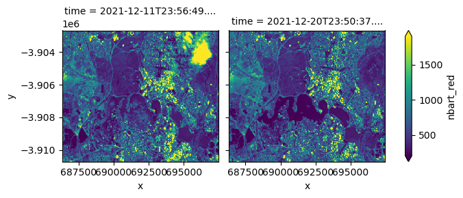
For example, we can filter by the eo:cloud_cover property to load only mostly cloud free observations (e.g. less than 10% cloud).
For more information about using filter, refer to the STAC guide here.
[9]:
# Set up a filter query
filter_query = "eo:cloud_cover < 10"

# Query with filtering
query = catalog.search(
    bbox=bbox,
    collections=collections,
    datetime=f"{start_date}/{end_date}",
    filter=filter_query,
)

# Load our filtered data
ds_filtered = odc.stac.load(
    query.items(),
    bands=["nbart_red"],
    crs="utm",
    resolution=30,
    groupby="solar_day",
    bbox=bbox,
)

# Plot our filtered data
ds_filtered.nbart_red.plot(col="time", robust=True);
Filtering can be performed on multiple metadata fields at once - for example, filtering by both cloud cover and geometric accuracy:
filter_query = "(eo:cloud_cover < 10) AND (gqa:abs_iterative_mean_xy < 1)"
Sorting
The DEA STAC API supports sorting results by metadata fields using the sortby extension parameter. For example, we can request that STAC items are returned in ascending order of cloud cover:
[10]:
# Query with sorting
query = catalog.search(
    bbox=bbox,
    collections=collections,
    datetime=f"{start_date}/{end_date}",
    sortby="eo:cloud_cover",
)

# Print out cloud cover values from low to high
[i.properties["eo:cloud_cover"] for i in query.items()]
[10]:
[0.7413425371604095,
 5.218904736222981,
 5.84303770341032,
 16.825931028459298,
 28.258366277957347,
 41.91683359769932,
 85.11645459806458,
 98.44253190598418]
Items can be sorted in descending order by prefixing the property name with -:
[11]:
# Query with sorting
query = catalog.search(
    bbox=bbox,
    collections=collections,
    datetime=f"{start_date}/{end_date}",
    sortby="-eo:cloud_cover",
)

# Print out cloud cover values from high to low
[i.properties["eo:cloud_cover"] for i in query.items()]
[11]:
[98.44253190598418,
 85.11645459806458,
 41.91683359769932,
 28.258366277957347,
 16.825931028459298,
 5.84303770341032,
 5.218904736222981,
 0.7413425371604095]
Fields
We can also restrict the metadata fields we load from the DEA STAC API using the filter extension parameter. This can be useful for more efficiently returning a small subset of fields from large volumes of metadata.
Metadata fields to load can be configured by passing in a dictionary with “include” and “exclude” keys. For example, we can choose to include only the odc:region_code and eo:cloud_cover metadata fields (note that we need to prefix these field names with properties.{}):
[12]:
# Query with sorting
query = catalog.search(
    bbox=bbox,
    collections=collections,
    datetime=f"{start_date}/{end_date}",
    fields={"include": ["properties.odc:region_code", "properties.eo:cloud_cover"]},
)

# Inspect returned STAC item properties
list(query.items())[0].properties
[12]:
{'datetime': '2021-12-04T23:50:39.744022Z',
 'eo:cloud_cover': 85.11645459806458,
 'odc:region_code': '090084'}
Additional resources
Explore the following Jupyter Notebooks for more in-depth guides to querying and loading data from STAC:
For more information about pystac_client and odc-stac: