DEA Land Cover (Landsat)
DEA Land Cover (Landsat)
- Version:
- Type:
Derivative, Raster
- Resolution:
30 m
- Coverage:
1988 to 2025
- Data updates:
Yearly frequency, Ongoing

About
Digital Earth Australia (DEA) Land Cover translates over 35 years of satellite imagery into evidence of how Australia’s land, vegetation, and waterbodies have changed over time.
This version includes breaking changes
All tile grid references have been changed to refer to a new origin point. Learn more in the Version 2.0.0 changelog.
Access the data
For help accessing the data, see the Access tab.
Key specifications
For more specifications, see the Specifications tab.
Technical name |
Geoscience Australia Landsat Land Cover 30m |
Bands |
|
DOI |
|
Currency |
|
Parent products |
DEA Water Observations (Landsat), DEA Water Observations Statistics (Landsat), DEA Fractional Cover (Landsat), DEA Fractional Cover Percentiles (Landsat), DEA Tasseled Cap Percentiles (Landsat), DEA Mangroves (Landsat), DEA Intertidal Elevation (Landsat) v1.0.0, GA SRTM 1 second DEM, Landsat 5, 7, 8, and 9 NBART and Observational Attributes |
Collection |
|
Licence |
Cite this product
Data citation |
Tissott, B., Mueller, N., Jorand, C., Ebadi, T., Ai, E., Kooymans, C., Harrison, M., Miller, J., Lucas, R., Metternicht, G., Owers, C.J., Clewley, D., Planque, C., Punalekar, S., Chua, S.M.T., Bunting, P., Lewis, B., Lymburner, L., Siggins, A, 2025. DEA Land Cover 30m. Geoscience Australia, Canberra. https://doi.org/10.26186/149976
|
Paper citation |
Lucas, R., Mueller, N., Siggins, A., Owers, C., Clewley, D., Bunting, P., Kooymans, C., Tissott, B., Lewis, B., Lymburner, L., Metternicht, G., 2019. Land Cover Mapping using Digital Earth Australia. Data. 4(4):143. https://doi.org/10.3390/data4040143
|
Publications
Lucas R, Mueller N, Siggins A, Owers C, Clewley D, Bunting P, Kooymans C, Tissott B, Lewis B, Lymburner L, Metternicht G. Land Cover Mapping using Digital Earth Australia. Data. 2019; 4(4):143. https://doi.org/10.3390/data4040143
Christopher J. Owers, Richard M. Lucas, Daniel Clewley, Carole Planque, Suvarna Punalekar, Belle Tissott, Sean M. T. Chua, Pete Bunting, Norman Mueller & Graciela Metternicht (2021) Living Earth: Implementing national standardised land cover classification systems for Earth Observation in support of sustainable development, Big Earth Data, 5:3, 368-390, DOI: 10.1080/20964471.2021.1948179
Background
Land cover is the observed physical cover on the Earth’s surface including trees, shrubs, grasses, soils, exposed rocks, water bodies, plantations, crops, and built structures. An Australia-wide land cover product provides an understanding of how the different parts of the environment change and interrelate. Earth observation data recorded consistently over a period of time allows the observation of the state of land cover at a specific time and also the way that land cover changes by comparison between times.
Use constraints
DEA Land Cover is appropriate to use at the national scale where other more detailed information on land cover is not available. Where DEA Land Cover’s data conflicts with state or local datasets, those datasets should be considered authoritative.
What this product offers
DEA Land Cover provides annual land cover classifications for Australia using the Food and Agriculture Organisation’s (FAO) Land Cover Classification System (LCCS) taxonomy Version 2 (Di Gregorio and Jansen, 1998; 2005).
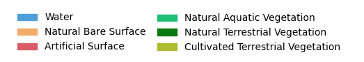
DEA Land Cover divides the landscape into six base land cover types, which are then further detailed through the addition of environmental descriptors (currently only accessible on DEA Maps). The structure is as follows.
Cultivated Terrestrial Vegetation
Percentage of cover
Life form (woody or herbaceous only)
Natural Terrestrial Vegetation
Percentage of cover
Life form (woody or herbaceous)
Natural Aquatic Vegetation
Percentage of cover
Life form (woody or herbaceous)
Water seasonality
Artificial Surfaces
Natural Bare
Percentage of bare cover
Water
Water persistence
Intertidal area
Applications
Annual Land Cover information can be used in a number of ways to support the monitoring and management of environments in Australia. These include, but are not limited to, the following areas of environmental monitoring, primary industries, and the interests and safety of the Australian community.
Environmental monitoring
Ecosystem mapping
Carbon dynamics
Erosion management
Agriculture Sector
Monitoring crop responses to water availability
Understanding drought impact on vegetation
Community interests
Map urban expansion within Australia
Mapping impacts of natural disasters
Bushfire recovery
Technical information
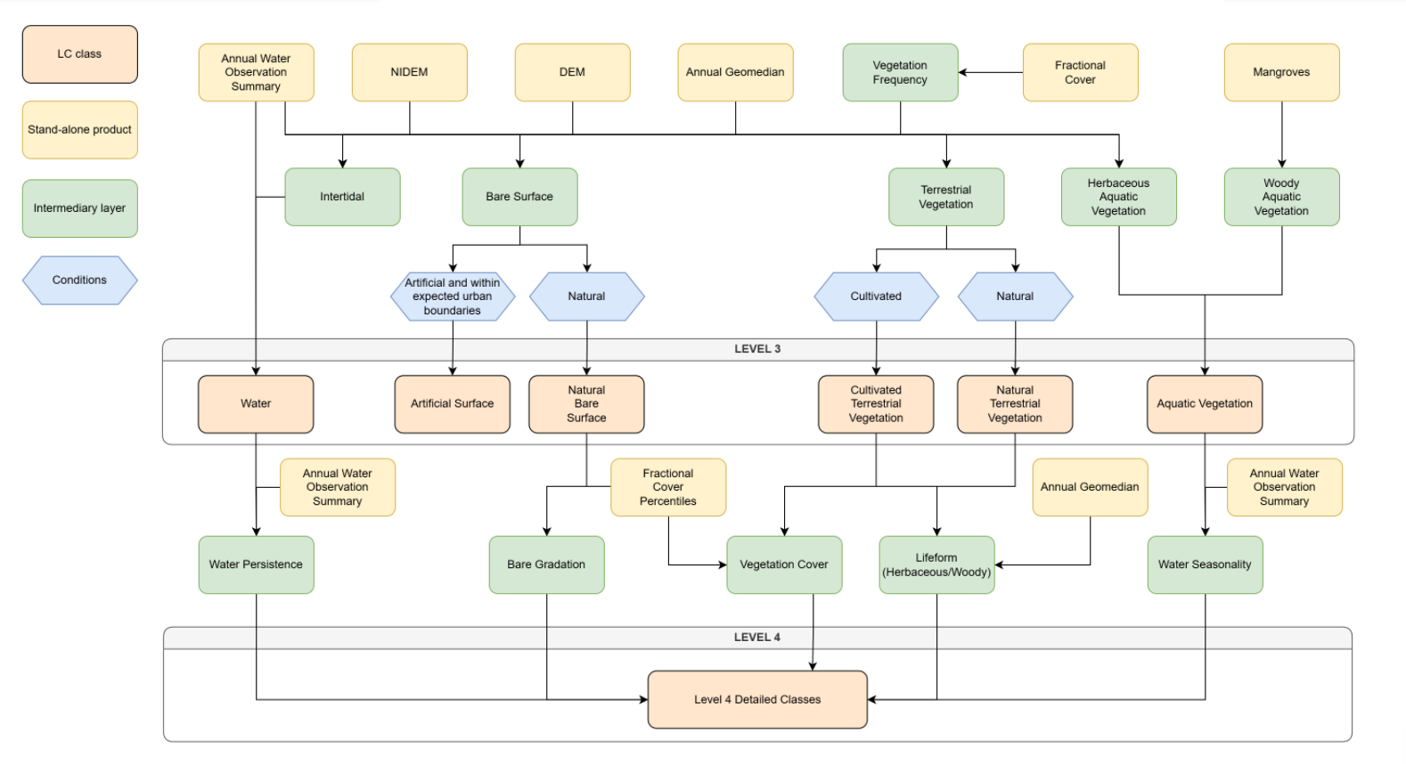
DEA Land Cover is based on the globally applicable Food and Agriculture Organisation’s (FAO) Land Cover Classification System (LCCS) taxonomy Version 2 (Di Gregorio and Jansen, 1998; 2005). DEA Land Cover classifications have been generated by combining quantitative (continuous) or qualitative (thematic) environmental information (referred to as Essential Descriptors; EDs) derived from Landsat satellite sensor data. Several EDs have been generated previously by Geoscience Australia, including annual water summaries (Mueller et al., 2016), vegetation fractional cover (Scarth et al., 2010), mangrove extent (Lymburner et al., 2020) and the Intertidal Extent Model (ITEM; Sagar et al., 2017), whilst others have been developed more recently. These EDs have been combined to generate detailed, consistent, and expandable annual classifications of Australia’s land cover from 1986 through to the present.
DEA Land Cover consists of two datasets: The base (Level 3) classification, and the final (Level 4) classification which combines the base classes with their associated descriptors.
Detailed layer descriptions, including known issues, are provided in the following sections.
Level 3
Classifications of Level 3
The base Level 3 land cover classification.
111:  Cultivated Terrestrial Vegetation (CTV)

112:  (Semi-)Natural Terrestrial Vegetation (NTV)

124:  Natural Aquatic Vegetation (NAV)

215:  Artificial Surface (AS)

216:  Natural Bare Surface (NS)

220:  Water

255: No data
Cultivated Terrestrial Vegetation (CTV)
Cultivated Terrestrial Vegetation (CTV) is associated with agricultural areas where active cultivation has been observed. In version 2.0, only herbaceous cultivation is shown and describes vegetation of strongly varying cover, ranging from bare (e.g. ploughed) areas to fully developed crops. Whilst the continental product describes land cover, interpretation is complicated as the same terminology is used to report on land use.
The definition of cultivated, and the difference from natural or semi-natural land covers, can be contentious, particularly as much of the Australian landscape is used for agricultural food production. This includes areas of Natural Terrestrial Vegetation (NTV) and Natural Aquatic Vegetation (NAV) that are grazed by stock and which can be regarded as either semi-natural or cultivated.
CTV in the DEA Land Cover map is associated with areas where management practices aimed at cultivation (including for grass production) are actively performed during the year being shown. These practices include crop planting and harvesting, fertilisation, and ploughing. These practices often lead to highly dynamic spectral signals within and between years but also regular transitions between vegetation of different cover amounts as well as bare soil. This also means that agricultural areas will transition between natural and cultivated covers as management practices transition an area between actively cropped or grazed, to areas left fallow, areas reduced to low cover due to climate effects such as drought, or to other covers depending on what the predominant conditions are through the year being shown.
Natural Terrestrial Vegetation (NTV)
Natural Terrestrial Vegetation (NTV) represents areas that have all or most of the characteristics of natural or semi-natural herbaceous or woody vegetation (based primarily on floristics, structure, function, and dynamics). These areas are identified as primarily vegetated, with either a photosynthetic vegetation fraction (PV) or non-photosynthetic fraction (NPV) greater than the bare soil fraction (BS) for at least two consecutive months. This approach considers that vegetation can exist in, and transition between PV and NPV states during the year. In effect, this approach classifies the landscape as primarily vegetated where the vegetated fraction of a pixel is greater than 30 %. Where the proportion of the landscape is less than 30 % vegetated, it is regarded as a sparsely vegetated or Natural Bare Surface, but the cover proportions can still be quantified. Urban areas that are vegetated (e.g. suburbs with trees) are associated with NTV if the pixel is at least 30 % vegetated but as Artificial Surfaces (AS) otherwise. The implementation allows areas of semi-natural vegetation (e.g. native grassland and pastureland) to be included in the NTV class.
Natural Aquatic Vegetation (NAV)
Natural Aquatic Vegetation (NAV) is associated primarily with wetlands that are dominated by woody or herbaceous vegetation (as with NTV). NAV is most commonly associated with mangroves, but may also include other forms of aquatic vegetation occurring within the maximum extent expected from mangroves.
Artificial Surfaces (AS)
Artificial Surfaces (AS) are areas of non-vegetated land cover created by human activities and are primarily represented by impervious surfaces (e.g. urban and industrial buildings, roads, and railways). These can be more readily identified when the area is larger than the spatial resolution (30 m) provided by the sensor. Open cut extraction sites are often included in AS. However, there is considerable misclassification of NS as AS in areas where vegetated cover is very low and very consistent through the year.
Natural Bare Surfaces (NS)
Natural Bare Surfaces (NS) are comprised primarily of unconsolidated (often pervious, e.g. mudflats and saltpans) or consolidated (e.g. bare rock or bare soil) materials. In Australia, the proportional area of Natural Bare Surfaces is relatively low and primarily confined to the deserts and semi-arid areas, river channels (e.g. dry riverbeds) and the coastline (e.g. mudflats and sand dunes). Much of the interior of Australia is sparsely vegetated and can be dominated by herbaceous (annual or perennial) or woody lifeforms.
Water
The Water class captures terrestrial and coastal open water such as dams, lakes, large rivers, and the coastal and near-shore zone.
Level 4
Classifications of Level 4
All categories from Level 3 and Level 4 algorithms are combined to give a single classification value for a given pixel.
The list below includes classes of different hierarchies, reflecting different levels of detail. The higher-level classes are used as fallback classes in cases where a confident detailed classification was not possible, and they are generally rare.
1:    Cultivated Terrestrial Vegetated

2:    Cultivated Terrestrial Vegetated: Woody

3:    Cultivated Terrestrial Vegetated: Herbaceous

4:    Cultivated Terrestrial Vegetated: Closed (> 65 %)

5:    Cultivated Terrestrial Vegetated: Open (40 to 65 %)

6:    Cultivated Terrestrial Vegetated: Open (15 to 40 %)

7:    Cultivated Terrestrial Vegetated: Sparse (4 to 15 %)

8:    Cultivated Terrestrial Vegetated: Scattered (1 to 4 %)

9:    Cultivated Terrestrial Vegetated: Woody Closed (> 65 %)

10:   Cultivated Terrestrial Vegetated: Woody Open (40 to 65 %)

11:   Cultivated Terrestrial Vegetated: Woody Open (15 to 40 %)

12:   Cultivated Terrestrial Vegetated: Woody Sparse (4 to 15 %)

13:   Cultivated Terrestrial Vegetated: Woody Scattered (1 to 4 %)

14:   Cultivated Terrestrial Vegetated: Herbaceous Closed (> 65 %)

15:   Cultivated Terrestrial Vegetated: Herbaceous Open (40 to 65 %)

16:   Cultivated Terrestrial Vegetated: Herbaceous Open (15 to 40 %)

17:   Cultivated Terrestrial Vegetated: Herbaceous Sparse (4 to 15 %)

18:   Cultivated Terrestrial Vegetated: Herbaceous Scattered (1 to 4 %)

19:   Natural Terrestrial Vegetated

20:   Natural Terrestrial Vegetated: Woody

21:   Natural Terrestrial Vegetated: Herbaceous

22:   Natural Terrestrial Vegetated: Closed (> 65 %)

23:   Natural Terrestrial Vegetated: Open (40 to 65 %)

24:   Natural Terrestrial Vegetated: Open (15 to 40 %)

25:   Natural Terrestrial Vegetated: Sparse (4 to 15 %)

26:   Natural Terrestrial Vegetated: Scattered (1 to 4 %)

27:   Natural Terrestrial Vegetated: Woody Closed (> 65 %)

28:   Natural Terrestrial Vegetated: Woody Open (40 to 65 %)

29:   Natural Terrestrial Vegetated: Woody Open (15 to 40 %)

30:   Natural Terrestrial Vegetated: Woody Sparse (4 to 15 %)

31:   Natural Terrestrial Vegetated: Woody Scattered (1 to 4 %)

32:   Natural Terrestrial Vegetated: Herbaceous Closed (> 65 %)

33:   Natural Terrestrial Vegetated: Herbaceous Open (40 to 65 %)

34:   Natural Terrestrial Vegetated: Herbaceous Open (15 to 40 %)

35:   Natural Terrestrial Vegetated: Herbaceous Sparse (4 to 15 %)

36:   Natural Terrestrial Vegetated: Herbaceous Scattered (1 to 4 %)

55:   Natural Aquatic Vegetated

56:   Natural Aquatic Vegetated: Woody

57:   Natural Aquatic Vegetated: Herbaceous

58:   Natural Aquatic Vegetated: Closed (> 65 %)

59:   Natural Aquatic Vegetated: Open (40 to 65 %)

60:   Natural Aquatic Vegetated: Open (15 to 40 %)

61:   Natural Aquatic Vegetated: Sparse (4 to 15 %)

62:   Natural Aquatic Vegetated: Scattered (1 to 4 %)

63:   Natural Aquatic Vegetated: Woody Closed (> 65 %)

64:   Natural Aquatic Vegetated: Woody Closed (> 65 %) Water > 3 months (semi-) permanent

65:   Natural Aquatic Vegetated: Woody Closed (> 65 %) Water < 3 months (temporary or seasonal)

66:   Natural Aquatic Vegetated: Woody Open (40 to 65 %)

67:   Natural Aquatic Vegetated: Woody Open (40 to 65 %) Water > 3 months (semi-) permanent

68:   Natural Aquatic Vegetated: Woody Open (40 to 65 %) Water < 3 months (temporary or seasonal)

69:   Natural Aquatic Vegetated: Woody Open (15 to 40 %)

70:   Natural Aquatic Vegetated: Woody Open (15 to 40 %) Water > 3 months (semi-) permanent

71:   Natural Aquatic Vegetated: Woody Open (15 to 40 %) Water < 3 months (temporary or seasonal)

72:   Natural Aquatic Vegetated: Woody Sparse (4 to 15 %)

73:   Natural Aquatic Vegetated: Woody Sparse (4 to 15 %) Water > 3 months (semi-) permanent

74:   Natural Aquatic Vegetated: Woody Sparse (4 to 15 %) Water < 3 months (temporary or seasonal)

75:   Natural Aquatic Vegetated: Woody Scattered (1 to 4 %)

76:   Natural Aquatic Vegetated: Woody Scattered (1 to 4 %) Water > 3 months (semi-) permanent

77:   Natural Aquatic Vegetated: Woody Scattered (1 to 4 %) Water < 3 months (temporary or seasonal)

78:   Natural Aquatic Vegetated: Herbaceous Closed (> 65 %)

79:   Natural Aquatic Vegetated: Herbaceous Closed (> 65 %) Water > 3 months (semi-) permanent

80:   Natural Aquatic Vegetated: Herbaceous Closed (> 65 %) Water < 3 months (temporary or seasonal)

81:   Natural Aquatic Vegetated: Herbaceous Open (40 to 65 %)

82:   Natural Aquatic Vegetated: Herbaceous Open (40 to 65 %) Water > 3 months (semi-) permanent

83:   Natural Aquatic Vegetated: Herbaceous Open (40 to 65 %) Water < 3 months (temporary or seasonal)

84:   Natural Aquatic Vegetated: Herbaceous Open (15 to 40 %)

85:   Natural Aquatic Vegetated: Herbaceous Open (15 to 40 %) Water > 3 months (semi-) permanent

86:   Natural Aquatic Vegetated: Herbaceous Open (15 to 40 %) Water < 3 months (temporary or seasonal)

87:   Natural Aquatic Vegetated: Herbaceous Sparse (4 to 15 %)

88:   Natural Aquatic Vegetated: Herbaceous Sparse (4 to 15 %) Water > 3 months (semi-) permanent

89:   Natural Aquatic Vegetated: Herbaceous Sparse (4 to 15 %) Water < 3 months (temporary or seasonal)

90:   Natural Aquatic Vegetated: Herbaceous Scattered (1 to 4 %)

91:   Natural Aquatic Vegetated: Herbaceous Scattered (1 to 4 %) Water > 3 months (semi-) permanent

92:   Natural Aquatic Vegetated: Herbaceous Scattered (1 to 4 %) Water < 3 months (temporary or seasonal)

93:   Artificial Surface

94:   Natural Surface

95:   Natural Surface: Sparsely vegetated

96:   Natural Surface: Very sparsely vegetated

97:   Natural Surface: Bare areas, unvegetated

98:   Water

99:   Water: (Water)

100:  Water: (Water) Tidal area

101:  Water: (Water) Perennial (> 9 months)

102:  Water: (Water) Non-perennial (7 to 9 months)

103:  Water: (Water) Non-perennial (4 to 6 months)

104:  Water: (Water) Non-perennial (1 to 3 months)

255: No data
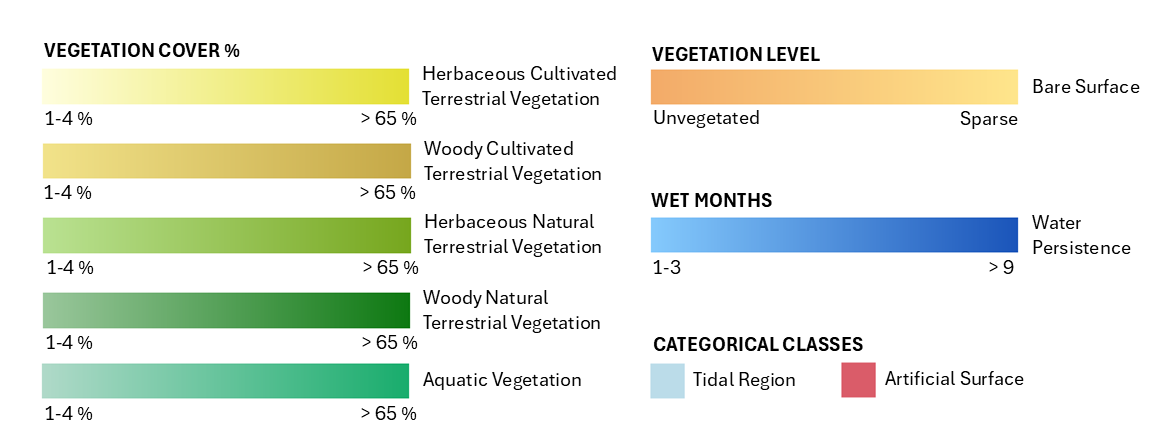
Lifeform (NTV, NAV, and CTV; 2 classes)
Lifeform represents the dominant vegetation type of a primarily vegetated area, discriminating woody from non-woody (herbaceous) vegetation. The Woody Cover Fraction models woody as vegetation of at least 20 % canopy cover. Hence the dominant vegetation in areas designated as woody in this product is considered to be composed of shrubs and trees. However, where woody vegetation is not dominant in an area, the cover will be essentially herbaceous or bare. Hence some areas containing sparse trees or shrubs will likely be represented as herbaceous.
Vegetation Cover (NTV, NAV, and CTV; 5 classes)
Vegetation Cover is defined using the statistics of annual fractional cover of PV (for a calendar year). This relates to the uppermost foliage as observed from the Landsat satellite sensor, and describes the percentage of an area that is vegetated rather than bare.
Water Seasonality (NAV; 2 classes)
Water Seasonality refers to the typical hydrological conditions in NAV within a year and is relevant to both coastal and inland wetlands. The current implementation utilises the DEA Water Observations (WO) dataset, identifying hydro-periods for NAV areas where water is somewhat permanent (over 3 months) or temporary or seasonal (under 3 months).
Water State (Water; 1 class)
Water State establishes whether water is present in liquid form or as snow or ice. The current product only identifies areas where water is present as liquid for at least 20 % of observations (based on WOfS).
Water Persistence (Water; 4 classes)
Water Persistence (or hydro-period) describes the maximum duration (in months) that water is seen to be covering the surface in the year.
Intertidal (Water; 1 class)
Intertidal water refers to primarily non-vegetated aquatic areas with systematic tidal water variations.
Natural Surface (NS; 3 classes)
Natural Surface (i.e., bare gradation) describes the percentage of bare surface in areas which contain sporadic or little persistent green vegetation through the year. The percentage reflects that much of the remaining area is brown or dead vegetation. This is characteristic of the more arid parts of Australia.
Lineage
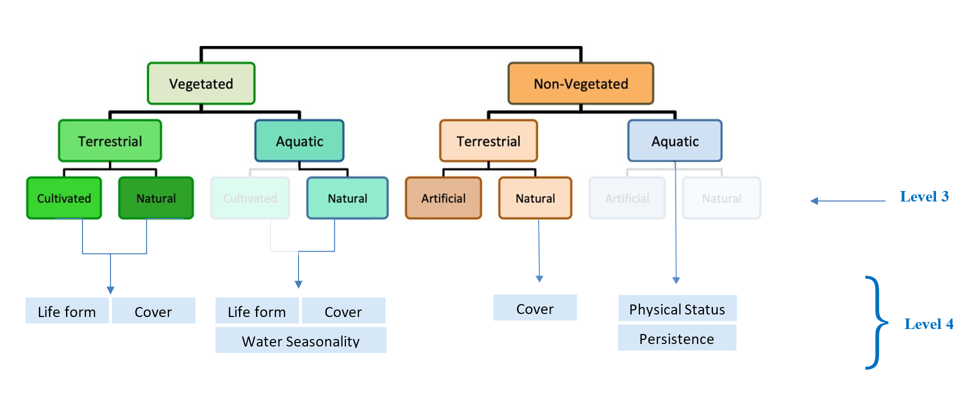
The FAO LCCS taxonomy (Figure 2) is hierarchical and consists of a dichotomous phase (Levels 1 to 3) and a modular phase (Level 4). In Level 1, vegetated and non-vegetated areas are first separated. These are then divided into terrestrial or aquatic categories to form Level 2. In the vegetated terrestrial category, cultivated and natural (including semi-natural) areas are differentiated. The non-vegetated category is further divided into Artificial Surface and Natural Surface. These non-vegetated Natural Surface include low vegetation cover and bare areas. This results in six base land cover categories (including the non-vegetated aquatic class from Level 2).
At Level 4, vegetated areas are further classified using information that differentiates lifeform (woody and herbaceous) and quantifies vegetation cover percent and water seasonality (for Natural Aquatic Vegetation). Natural Surface areas have information added (bare gradation) which describes the level of remaining vegetation present (sparse, very sparse, or not detectable). Non-vegetated aquatic areas (Water) are further described on the basis of their persistence (hydro-period) over a calendar year. The FAO LCCS differentiates water in different physical states (liquid or frozen; ice or snow); however, only liquid water is included in the current release.
Software
References
Lucas R, Mueller N, Siggins A, Owers C, Clewley D, Bunting P, Kooymans C, Tissott B, Lewis B, Lymburner L, Metternicht G. Land Cover Mapping using Digital Earth Australia. Data. 2019; 4(4):143. https://doi.org/10.3390/data4040143
Christopher J. Owers, Richard M. Lucas, Daniel Clewley, Carole Planque, Suvarna Punalekar, Belle Tissott, Sean M. T. Chua, Pete Bunting, Norman Mueller & Graciela Metternicht (2021) Living Earth: Implementing national standardised land cover classification systems for Earth Observation in support of sustainable development, Big Earth Data, 5:3, 368-390, DOI: 10.1080/20964471.2021.1948179
Metternicht, G., Mueller, N., Lucas, R., Digital Earth for Sustainable Development Goals, Manual of Digital Earth, pp 443 - 471, Springer Singapore. https://doi.org/10.1007/978-981-32-9915-3_13
Limitations
DEA Land Cover is created by combining multiple layers that each describe features in the landscape. In doing so, the extents of each layer do not necessarily completely align, and some no-data points can cross between outputs. As a result, there are some Level 4 classes that only report detail to Level 3, as the details of cover fraction and water persistence do not have corresponding data in the respective datasets. This specifically relates the classes of Water, Natural Bare Surfaces, and Natural Aquatic Vegetation in areas near water bodies and the intertidal zone; however, the number of affected pixels is small.
Level 3 Class limitations
Cultivated Terrestrial Vegetation (CTV)
Managed plantations and some orchards and tree crops are not currently distinguishable from semi-natural or natural terrestrial vegetation and are not yet incorporated in the area of CTV. Reference can be made to Australia’s National Plantation Inventory. When savannah, semi-arid, and arid regions experience alternating browning and greening (as can occur due to fires, inundation, drought, and rainfall), this resembles the cyclical changes of cultivated land. This can cause areas of Natural Terrestrial Vegetation (NTV), Natural Bare Surfaces (NS), or Natural Aquatic Vegetation (NAV) to be misclassified as CTV. For example, the anomalously high levels of rainfall in 2010 led to some vegetation growth patterns that were classified as cultivated vegetation and these false positives reduced the precision of the class in that year. Several natural vegetation types, particularly in the monsoonal north, are misclassified as CTV due to burning, which can be associated with the indigenous management cycle. Saltmarshes, surface algae on mudflats, and aquatic vegetation on ephemeral inland floodplains can also be misclassified. Areas of bare soil exposed for long periods during the agricultural cycle or management activities and sparse vegetation (when areas are not in use or fallow such as during drought periods) can be misclassified as NS. This occurs particularly where areas have experienced low cover for prolonged periods within a year. The CTV machine learning algorithm has not been trained on CTV-woody areas, due to a lack of available training data, potentially leading to higher misclassification rates in these areas.
Natural Terrestrial Vegetation (NTV)
The NTV category can transition into the NS category between years when a highly variable Landsat satellite spectral signature is observed due to changes in vegetation productivity and moisture content. The transition of NTV to NS is particularly evident when comparing periods with rainfall above or below the average (e.g. 2010 was above; whereas, 2015 was below). Some confusion between surfaces that are primarily bare surfaces and non-photosynthetic vegetation remains and is also partly a function of the spectral reflectance of the underlying soil type. Vegetated areas shadowed by terrain can also be misclassified as non-vegetated. Areas of very low vegetation coverage are associated with the NS rather than NTV category, with the cover percentages shown as percentage bare. The assignment of vegetated suburbs to NTV is largely correct, but Artificial Surfaces (AS) located beneath the canopy are not currently represented in the product. Some confusion between CTV and NTV can occur because of natural seasonal changes in native vegetation. The edges of salt lakes may be misclassified as NTV.
Natural Aquatic Vegetation (NAV)
At Level 3, Natural Aquatic Vegetation (NAV) is represented as a merged class and does not distinguish between woody and herbaceous vegetation types. As a result, mangroves are the dominant vegetation type mapped within this class. However, other forms of natural aquatic vegetation may also be classified as NAV where they occur within the extent typically expected for mangroves.
Artificial Surfaces (AS)
The Artificial Surfaces machine learning algorithm works best in dense urban areas. Misclassification occurs with Natural Bare Surfaces (NS), particularly in arid and semi-arid regions, open cut mine sites, salt lakes and pans, sand dunes, and beaches. This is attributed to similarities in the variance of spectral signatures over a year. The Australian Bureau of Statistics - Urban Centre and Locality mask is applied to reduce some of these misclassifications in rural areas. Urban areas with high concentrations of surrounding vegetation may not be correctly classified as AS. Misclassification occurs in some cultivated areas due to the predominance of sparse vegetation, or when land is left fallow for most of the year. Cloud and data quality issues can lead to the incorrect assignment of other land cover classes to AS, such as in south-west Tasmania. Within dense urban centres with high-rise buildings such as the central business districts of Sydney or Melbourne, some areas are misclassified as Water due to the shadows of the high rise buildings. In some industrial areas, buildings can be misclassified as no data due to the bright surface reflectance having a similar signature to cloud.
Natural Bare Surfaces (NS)
Land used for agriculture may be associated with the NS class if ploughing or tillage has occurred and the vegetation cover remains low during the calendar year. Areas mapped as NS may temporarily transition to or from CTV under certain circumstances (e.g. during drought). This occurs because of the predominance of temporary vegetation (e.g. short crop life spans), desiccation, removal during dry periods, or management practices (e.g. land left as fallow). Where acquisition of cloud-free Landsat satellite sensor data has been infrequent, less information on the inter-annual variability of vegetation is provided. Where cloud cover is extensive (e.g. in Tasmania), the number of scenes for land cover classification is reduced and this can compromise classification of NS, particularly where bare surfaces alternate with vegetation. Confusion between natural surfaces and urban areas occurs because of similar spectral variation over an annual period.
Water
Areas of artificial and natural water are not differentiated, although the extent of artificial water is mapped within the existing Bureau of Meteorology Geofabric product. Due to the 30 m pixel size, rivers and water courses that cover less than a pixel, or with highly vegetated riverbanks are not captured. This results in a patch-like representation of narrower rivers. Areas of dark, wet soil are often misclassified as water, including in cultivated areas and mud flats. Some pixels surrounding water bodies have no classification, due to having no valid data from the Fractional Cover product, and the Water Observations product being unable to determine if the pixels are wet or dry. Classification of pixels over the ocean should not be used from Land Cover — the water persistence is often incorrect, and the land cover classification should be applied to land-only pixels. This Land Cover product should be used with an ocean mask for coastal tiles.
Level 4 Class limitations
Lifeform
Woody discrimination is implemented using the Woody Cover Fraction product (Liao et al, 2020) which models woody cover from inputs of LiDAR including ICESat/GLAS, L-band SAR, field observation, and Landsat satellite data. Issues arise in this dataset in areas dominated by short, woody vegetation such as heathland, and swampy regions with underlying water. Areas of woody savannah are also under-represented due to the influence of the herbaceous underlying cover dominating the observation.
A distinction between woody and herbaceous vegetation within NAV is introduced at Level 4. At this level, woody NAV corresponds to mangroves. Non‑woody (herbaceous) NAV may also be present within the maximum extent in which mangroves can occur. However, the herbaceous NAV has not been independently validated. Consequently, its presence and spatial distribution should be interpreted with caution.
Vegetation Cover
The cover of vegetation is derived from the Fractional Cover product (Scarth et al, 2010), and as such it reflects the limitations of that product, mainly difficulty with measurement of non-photosynthetic vegetation, and noise due to the presence of water in a pixel. Therefore, arid areas can be difficult to fully analyse for cover, leading to misclassifications between NTV, NS, and CTV where cover is sparse (lower than 15 %).
Water Seasonality
This product does not yet identify consecutive months but rather the frequency of wet observations in the year, based on the Water Observations product. Therefore, monthly statements are unlikely to be consistent across the continent. Water beneath mangroves cannot be easily observed due to their dense canopies. Hence, the hydro-period (and seasonality metrics) should be treated with some caution.
Water State
Mapping of ice and snow states is yet to be undertaken. Hence the Water State class is currently limited to liquid only.
Intertidal
The intertidal areas carry the limitations of the DEA Intertidal Extents (Landsat) product:
Intertidal areas are determined as a coastal mask, which currently identifies some non-tidal inland water bodies as tidal because of intra-annual changes in water extent.
This product is static and cannot be used to demonstrate change between two annual continental products.
Bare Gradation
The Bare Gradation class is produced from the Fractional Cover product. Unlike the Vegetation Cover class, Bare Gradation is calculated from the median bare fraction, rather than consecutive monthly green and non-photosynthetic fractions. As such the bare fraction can be as low as 20%, however this does not imply that the remaining fraction is healthy vegetation. Rather, the remaining fraction is a mix of brown, dead, and green vegetation, with intermittent green periods through the year, reflective of arid area vegetation types.
Earth Observation limitations
To generate the land cover classification for each calendar year, annual (January to December) statistics derived from Landsat-5, -7, -8, and -9 observations are currently used, with each satellite sensor potentially observing the Australian landscape every 16 days. This brings an intrinsic limitation to land cover mapping as persistent cloud in some regions reduces the number of useable observations. This is particularly evident in Tasmania, and northern Australia during the monsoon period, where areas may not be observed for extended periods and parts or all of the intra-annual land cover cycle may be missed due to persistent cloud. These limitations can lead to misclassifications of land cover, particularly in dynamic environments. In a future release, a confidence layer will be included to help identify areas with poor observation frequency or other factors impacting the classification.
An additional limitation of the Landsat series is the availability of data due to the ageing of each satellite. Landsat 5 was operational for over 25 years, but for much of the later years, data were only acquired when sunlight directly illuminated its solar panels. This limited its operation across Australia, with coverage being seasonally dependent, and contracting north to a minimum in winter. In its last years, the winter coverage usually only covered the northern coasts of Australia. Landsat 5 ceased regular operations over Australia in 2011, leaving just Landsat 7 operational until Landsat 8 was launched in 2013. Landsat 7 began service in 1999 as a replacement for Landsat 5. Initially Landsat 5 was switched off, but when Landsat 7 suffered a serious problem in 2003 due to the failure of its scan-line corrector (termed SLC-Off), Landsat 5 resumed service. The SLC-Off failure of Landsat 7 resulted in severe striping across every image from mid-2003 onwards, and this striping is apparent in subsequent derived products. Landsat 8 has operated well since its launch in 2013. Landsat 9 has operated since 2022 with improved sensitivity, noise characteristics, and data correction in comparison to the earlier sensors.
The result of the availability of these satellites is that the most consistent data availability occurs when two satellites are in operation (which occurred in most of the 2003 to present period). The least data availability is in 2011 to 2012 when only Landsat 7 was available, and its data quality was impaired by the SLC-Off striping issue. The overall data availability for the Landsat satellites is shown in Table 1. The datasets used in this analysis are shown in Table 2.
Years |
Satellite and sensor |
Issues |
Impact on LCCS product |
|---|---|---|---|
1986 |
Landsat 5 Thematic Mapper (TM) |
Only part of the year available in DEA. |
Very little data available. Year is omitted. |
1987 to 1999 |
Landsat 5 TM |
Normal operation |
Only single source of data is available. |
1999 to early 2003 |
Landsat 5 TM |
Switched off with availability of Landsat 7. |
Only single source of data is available. |
1999 to early 2003 |
Landsat 7 Enhanced Thematic Mapper (ETM+) |
Normal operation. |
Only single source of data is available. |
Late 2003 to early 2011 |
Landsat 5 TM |
Gradually degrading operation and increasing observation failure. Total failure in early 2011. |
Landsat 5 with Landsat 7 to fill in missed areas (clouds). |
Late 2003 to present |
Landsat 7 ETM+ |
Operating with SLC-Off stripes in imagery. |
Fill in for missed areas in Landsat 5 and 8. Only data available from early 2011 to early 2013. |
Early 2013 to present |
Landsat 8 Optical Land Imager (OLI) |
Normal operation. |
Landsat 8 with Landsat 7 to fill in missed areas (clouds). |
Product |
Used for |
Dataset reference |
|---|---|---|
Fractional Cover (FC) |
Vegetation |
Scarth et al. (2010), Schmidt et al. (2010) |
Water Observations from Space (WOfS) |
Aquatic |
Mueller et al. (2016) |
National Intertidal Digital Elevation Model (NIDEM) |
Aquatic |
Bishop-Taylor et al. (2018) |
National Mangrove extent |
Aquatic |
Lymburner et al. (2019) |
Machine learning applied to annual geometric medians (geomedians) and Median Absolute Deviations (MADs) |
Cultivated |
Roberts et al. (2017) (geomedians and MADs); Chua (cultivated) DEA (in draft) |
Machine learning applied to geomedians, MADs, and Woody Cover Fraction |
Artificial surfaces |
Tan and Chua, DEA (in draft) |
Woody Cover Fraction (WCF) |
Lifeform |
Liao et al. (2020) |
Accuracy
A validation assessment has been undertaken for both of the versions of Land Cover: the former Collection 2 (C2; i.e. Version 1), and the current Collection 3 (C3; i.e. Version 2). The below section outlines the accuracy of both versions to assist users in understanding the differences between them. The validation metrics reported were produced for Level 3 and they integrate the results from the validation of the sub-components of Level 1, the Artificial Surface model, and the Cultivated Terrestrial Vegetation model.
Summary of differences between Land Cover C2 and C3
Collection 3 generally aligns with Collection 2 in terms of classification performance, with trends across time periods and classes being mostly consistent. However, some deviations from this pattern have been observed across different locations and times, particularly in the CTV class.
Collection 3 classification shows better overall consistency across different validation methods.
An improvement in AS classification was observed in C3. More urban areas appear to be correctly identified, although there is a slight increase in false positive identification of urban areas in the central Australian desert and other sandy regions.
Slight improvement is seen in Woody Cover for the NTV classification.
There is a substantial increase in Landsat 7 stripe artefacts in C3 due to Landsat 8 scenes being filtered out due to poor geometric quality assessments.
There is a general increase in the number pixels with no data surrounding water bodies in C3.
Misclassification of water persistence over the ocean is observed in C3.
Collection 2 validation
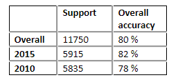
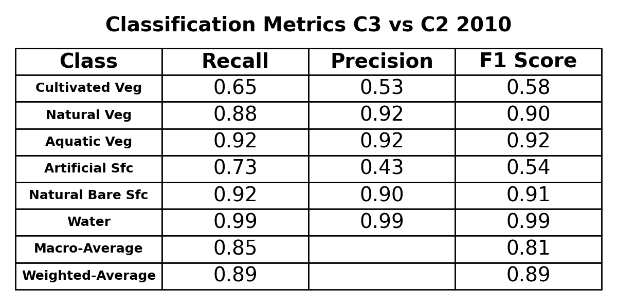
The product was validated using 6,000 points spatially distributed across Australia for the years 2010 and 2015, resulting in a total of 12,000 samples. These points were created using a stratified random sampling approach that was adjusted for oversampling. After removing points with ‘No Data’ and spurious values, the total number of valid points was 11,750. The sample points were divided into clusters for visual assessment against the classification outputs and individually assessed by a pool of 10 people. To compare individual biases among the assessors, an additional set of validation points was created and evaluated by all assessors. Table 3 contains the overall accuracy for all classes. The term ‘support’ refers to the number of validation points used in the calculation of that accuracy value.
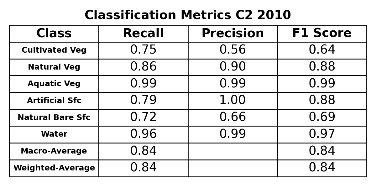
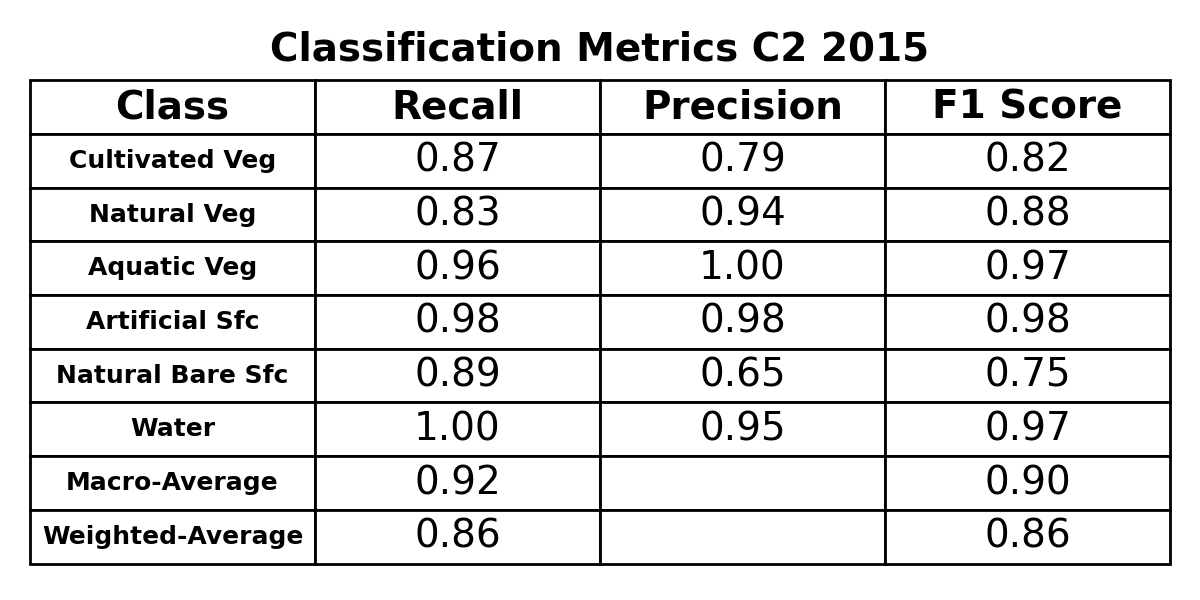
The results, shown in Table 4, also provides per-class accuracy information. ‘Precision’ refers to the ability of a classification model to return only relevant instances, while ‘Recall’ refers to the ability to identify all relevant instances. The ‘F1 score’ combines precision and recall to provide an overall measure of accuracy. Classes such as Artificial Surfaces (AS), Natural Aquatic Vegetation (NAV), and Water exhibited high accuracies. However, classifying Cultivated Terrestrial Vegetation (CTV) and Natural Bare Surfaces (NS) proved challenging, resulting in the lowest accuracies among the six classes presented.
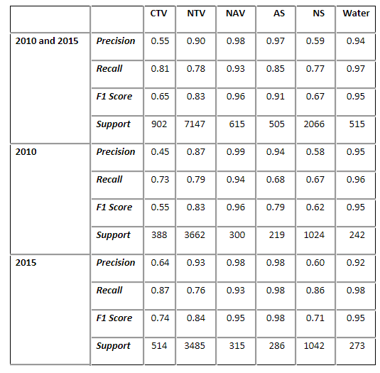
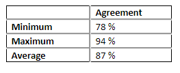
Table 5 indicates that where assessors could identify a predominant land cover (i.e., not ‘mixed’ pixels or ‘unsure’), there was 75% agreement among all assessors.
Collection 3 validation
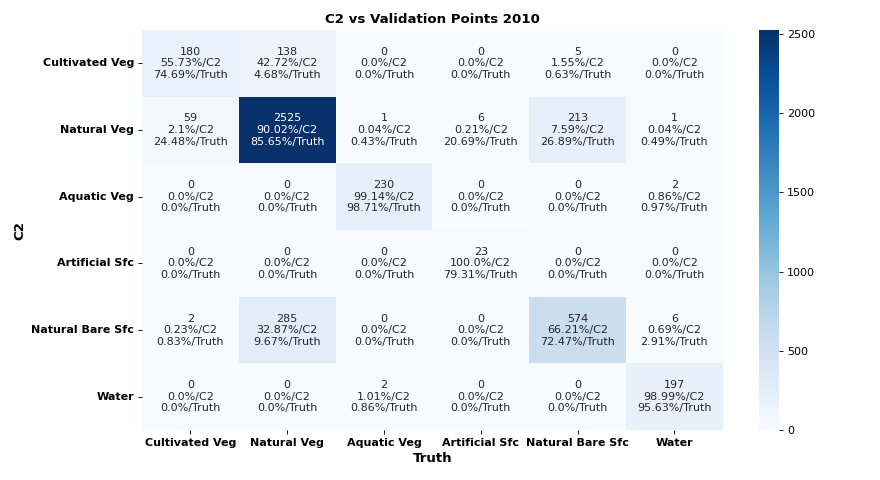
To understand the extent of change between the versions, validation against three data sources was undertaken. These were the validation points reused from Collection 2, with the addition of point attributes from Köppen Climate Zone and State/Territory to facilitate segment analysis; the GLANCE (Global Land Cover Estimation) global dataset of independent “ground truth” data; and the Land Cover Collection 2 data.
To account for the additional validation points, the Collection 2 (C2) validation was rerun and compared with the results from Collection 3 (C3).
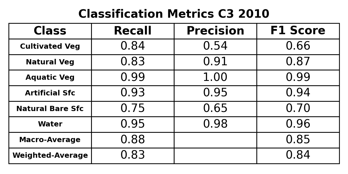
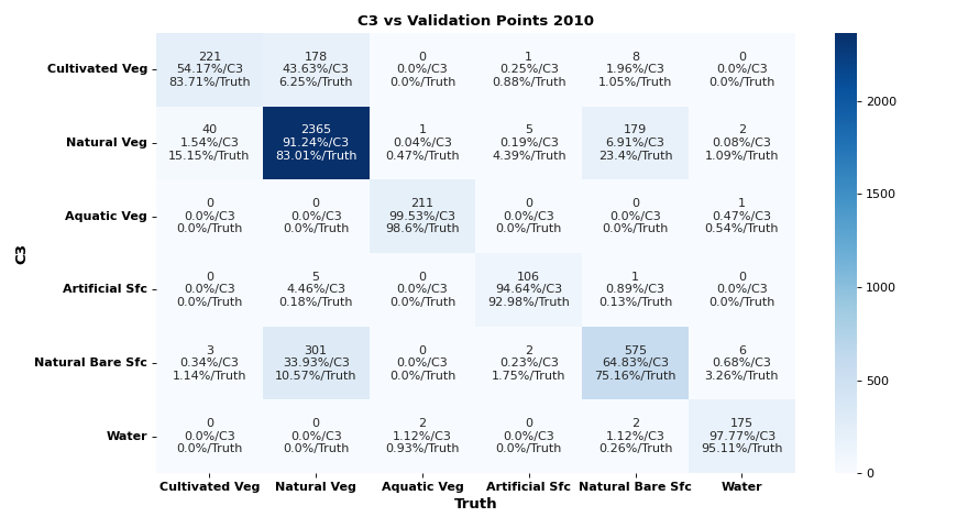
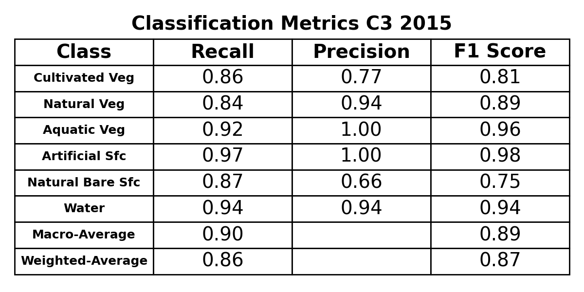
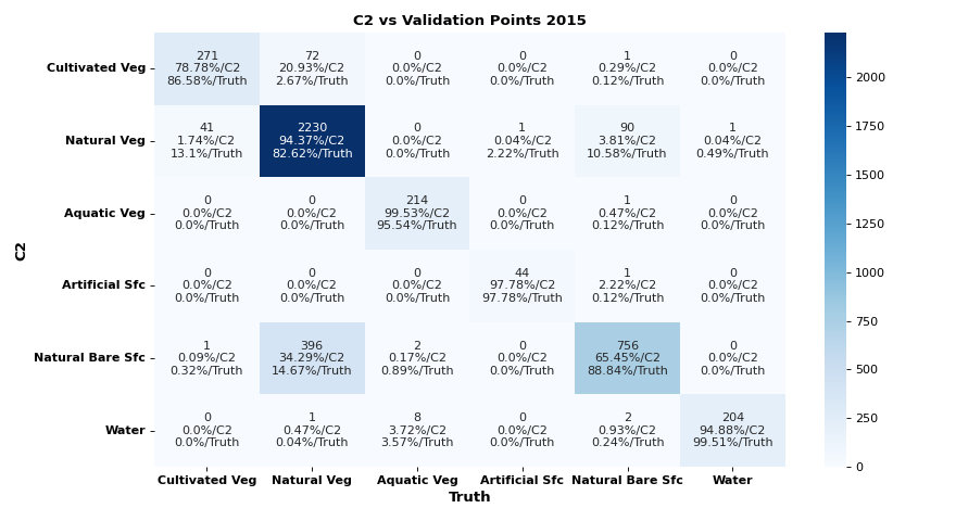
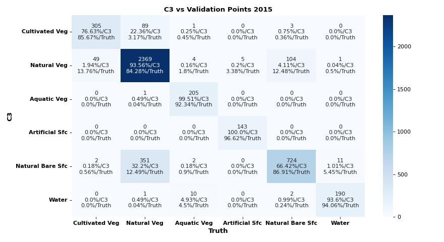
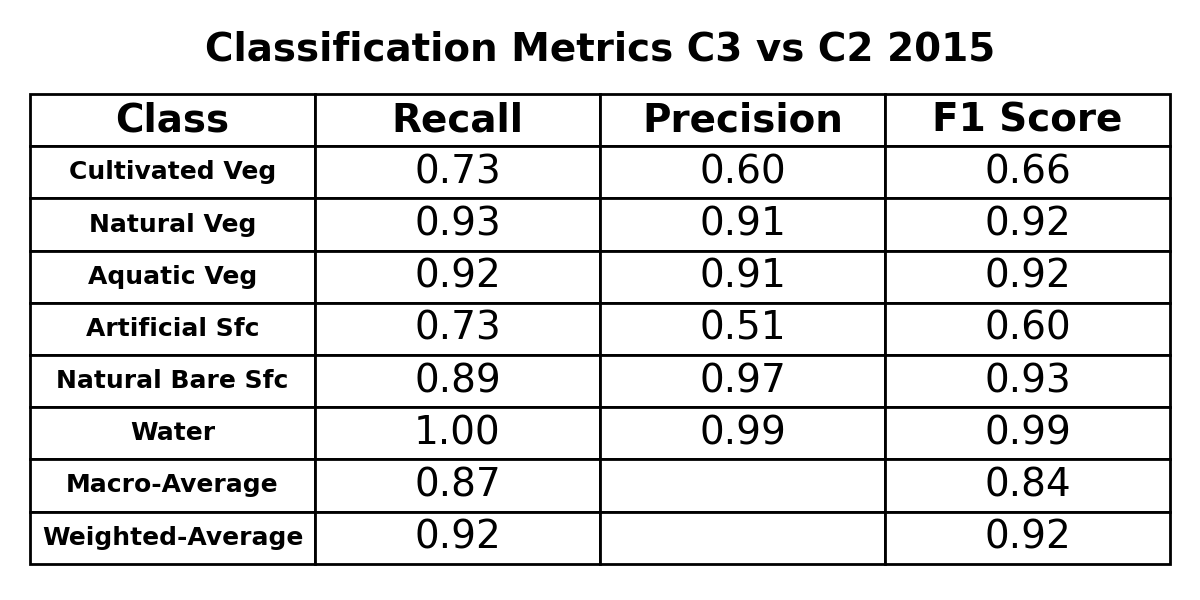
Both C3 and C2 showed overall degradation in 2010 compared to 2015, a trend propagated from the Level 1 and individual ML models results. The performance metrics with the validation points show an overall alignment of the two collections, with minimal differences across categories, except for the Recall values of Cultivated Terrestrial Vegetation (CTV) and Artificial Surface (AS), which are both higher in C3 for the year 2010 (see Tables 6 and 9).
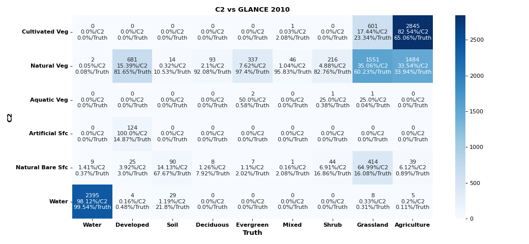
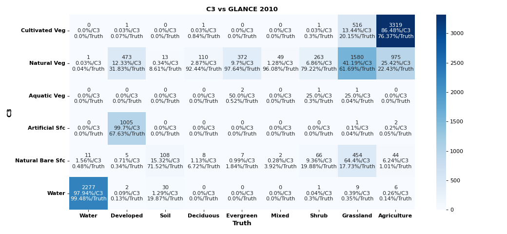
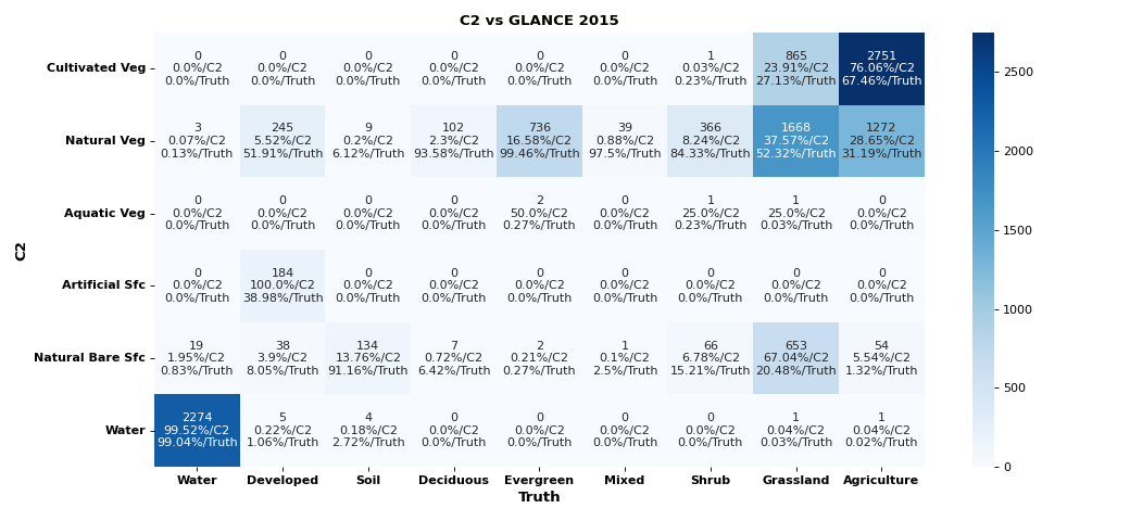
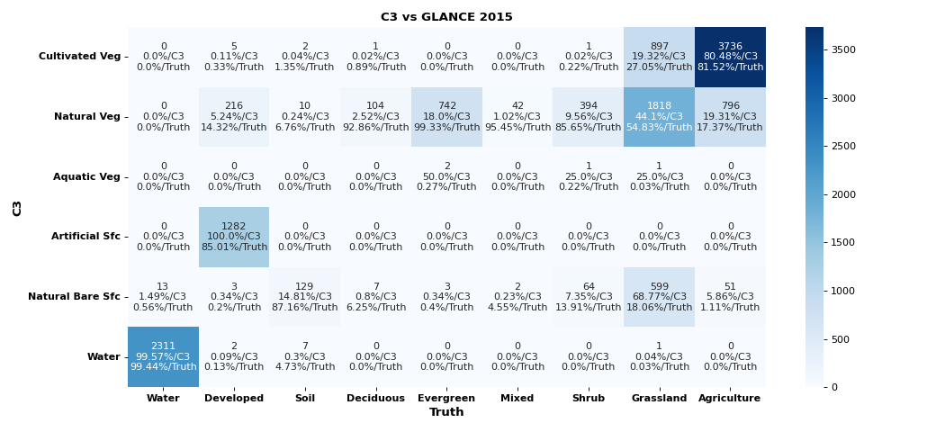
C3 demonstrated a more reasonable classification on the GLANCE dataset, particularly for the Natural Terrestrial Vegetation (NTV) class, which can be intuitively interpreted as the Agriculture category of the GLANCE dataset (see Tables 7, 8, 10, and 11).
C3 exhibited better consistency in results against the validation points and the GLANCE data. However, some misalignment between ground truth datasets is present in both collections for certain classes (e.g. Natural Bare Surfaces; NS). Some classes, such as Artificial Surface (AS), have too few validation points to be considered statistically significant. Hence, the classification metrics should be interpreted with caution and understood in relative terms, as a way to highlight the differences between C2 and C3, rather than the absolute performance of each.
When C3 was compared directly with the output of C2 (Table 16), it showed good agreement for most of the Level 3 classes. Two notable exceptions were the Cultivated Terrestrial Vegetation (CTV) class and the Artificial Surface (AS) class. For CTV, the performance against the validation data did not suggest a substantial difference in overall accuracy between C2 and C3; thus, the misalignment observed in Table 16 could be due to possible inconsistencies in classification between the two collections, but not necessarily an improvement or degradation. The difference observed in the AS classification may be influenced by the increased accuracy of C3.
In the classification metrics tables below, two types of averages are used to summarise the performance across different classes: Macro-Average and Weighted-Average. The Macro-Average is the unweighted mean of each metric, calculated independently for all classes. Each class contributes equally, regardless of its frequency in the dataset. This average should be interpreted as ‘unbiased’ due to the highly skewed nature of the validation points. The Weighted-Average, on the other hand, is the average of each metric weighted by the support (\(TP + FN\); i.e., True Positives and False Negatives) for each class. The weight reflects the proportion of each class in the ‘Truth’, meaning that more frequent classes have a greater impact on the overall average.
Validation points 2010
Validation points 2015
GLANCE 2010
GLANCE 2015
Collection 3 vs Collection 2
Product ID
The Product ID is ga_ls_landcover_class_cyear_3. This ID is used to load data from the Open Data Cube (ODC), for example dc.load(product="ga_ls_landcover_class_cyear_3", ...)
Bands
Bands are distinct layers of data within a product that can be loaded using the Open Data Cube (on the DEA Sandbox or NCI) or DEA’s STAC API.
Type |
Units |
Resolution |
No-data |
Aliases |
Description |
|
|---|---|---|---|---|---|---|
level3 |
uint8 |
- |
30 m |
255 |
- |
The base Level 3 Land Cover classification. |
level4 |
uint8 |
- |
30 m |
255 |
full_classification
|
All Level 3 and Level 4 classes are combined to give a single classification value. |
For more information on these bands, see the Description tab.
Product information
This metadata provides general information about the product.
Product ID |
ga_ls_landcover_class_cyear_3
|
Used to load data from the Open Data Cube. |
Short name |
DEA Land Cover (Landsat) |
The name that is commonly used to refer to the product. |
Technical name |
Geoscience Australia Landsat Land Cover 30m |
The full technical name that refers to the product and its specific provider, sensors, and collection. |
Version |
2.0.0 |
The version number of the product. See the History tab. |
Lineage type |
Derivative |
Derivative products are derived from other products. |
Spatial type |
Raster |
Raster data consists of a grid of pixels. |
Spatial resolution |
30 m |
The size of the pixels in the raster. |
Temporal coverage |
1988 to 2025 |
The time span for which data is available. |
Update frequency |
Yearly |
The expected frequency of data updates. Also called ‘Temporal resolution’. |
Update activity |
Ongoing |
The activity status of data updates. |
Currency |
Currency is a measure based on data publishing and update frequency. |
|
Latest and next update dates |
See Table B of the report. |
|
DOI |
The Digital Object Identifier. |
|
Catalogue ID |
The Data and Publications catalogue (eCat) ID. |
|
Licence |
See the Credits tab. |
Product categorisation
This metadata describes how the product relates to other products.
Access the data
DEA Maps |
Learn how to use DEA Maps. |
|
Digital Atlas applications |
Learn how to use the Land Cover Explorer. |
|
DEA Explorer |
Learn how to use the DEA Explorer. |
|
Data sources |
Learn how to access the data via AWS. |
|
Code examples |
Learn how to use the DEA Sandbox. |
|
Web services |
Learn how to use DEA’s web services. |
|
Digital Atlas Layers |
Learn how to create a map using Digital Atlas. |
How to view DEA Land Cover in a web map
To view and access the data interactively, follow these steps.
Visit DEA Maps.
Click Explore map data.
Click Land and vegetation > DEA Land Cover > DEA Land Cover (Landsat).
Click Add to the map, or the ‘+’ symbol to add the data to the map.
How to load DEA Land Cover with Python in the DEA Sandbox (Recommended)
DEA Sandbox allows you to explore DEA’s Earth Observation datasets in a JupyterLab environment. See the guide to get started with the DEA Sandbox.
Once you have signed up to the Sandbox, click into the DEA products directory to find the Introduction to DEA Land Cover notebook. This notebook will walk you through loading and visualising the DEA Land Cover data.
How to stream DEA Land Cover continental mosaics in QGIS or ESRI ArcGIS Pro from AWS (Recommended)
The easiest way to access DEA Land Cover data is via our continental-scale cloud-optimised GeoTIFF mosaics (COGs).
The COG file format is a type of GeoTIFF raster file (.tif) that allows you to quickly and efficiently ‘stream’ data directly from the Amazon S3 cloud without having to download files to your computer.
This allows you to rapidly access data from the entire Australian continent without having to download large files.
VRT (Virtual Raster) files are also provided alongside the .tif mosaics. These files serve as lightweight wrappers around the main data and can be used to open data in GIS software with visual settings already applied.
For detailed instructions, please visit the Continental Cloud-Optimised GeoTIFF Mosaics page
How to integrate DEA Land Cover continental mosaics into your own Python workflow
You can seamlessly open a Land Cover mosaic, such as Level 4 for year 2024, using Python and the rioxarray library. For example:
import rioxarray
cog_url = 'https://data.dea.ga.gov.au/derivative/ga_ls_landcover_class_cyear_3/2-0-0/continental_mosaics/2024--P1Y/ga_ls_landcover_class_cyear_3_mosaic_2024--P1Y_level4.tif'
cog = rioxarray.open_rasterio(cog_url, chunks=True)
This loads the remote dataset directly into an xarray DataArray. At this point, you can continue analysing the data as you would with any other raster array.
How to download DEA Land Cover data via web browser
From DEA’s public data (ga_ls_landcover_class_cyear_3), navigate through the folders to the year and tile of interest, then click the GeoTIFF file of the relevant layer to download it directly.
To find the X and Y tile values for a particular area, you can use the DEA Explorer.
How to download DEA Land Cover data via AWS
DEA Land Cover data can be downloaded in bulk using Amazon Web Service’s Command Line Interface (AWS CLI). This method is for technical users.
You can now download data from the command line using a command such as this example which downloads all level4 tiles for 2020 into a folder called ‘landcover’. You will need to modify the command based on your particular use case.
aws s3 --no-sign-request sync s3://dea-public-data/derivative/ga_ls_landcover_class_cyear_3/2-0-0/2020 C:/landcover/ --exclude "*" --include "*_level4.tif"
In this command,
The S3 bucket and folder to download data from is
s3://dea-public-data/derivative/ga_ls_landcover_class_cyear_3/2-0-0/2020The directory to download to is
C:/landcover/When you want to specify specific files to download, first you need to exclude everything, then you can define which files to include:
--exclude "*" --include "*_level4.tif"
How to add DEA Land Cover to QGIS using the OWS web service
Note: You must be using QGIS version 3.22 or above to use the time dimension.
From the top menu bar, click Layer > Add Layer > Add WMS/WMTS Layer.
Click New to set up a new data source, then enter the following.
Name:
DEA ServicesURL:
https://ows.dea.ga.gov.au/
Click Connect.
Once the items appear, you can choose which layers to add.
Click Land and Vegetation > DEA Land Cover Collection 3, then select either of the following options.
DEA Land Cover Collection 3 Calendar Year (Landsat), then select either Basic or Detailed.
DEA Land Cover Environmental Descriptors, then select any of the various descriptor layers (Lifeform, Water Seasonality, etc.)
Click Add.
How to add DEA Land Cover to QGIS using GeoTIFF tiles (Not recommended)
Individual tiles can be downloaded via web browser or AWS by following the above instructions and can then be uploaded to QGIS.
The QGIS style files can be downloaded from the following locations.
To add the style to QGIS, do the following.
Select the TIF files you would like the styling applied to.
Right-click that selection then select Properties > Symbology.
In the bottom left menu, click Style > Load Style.
The styling will now be applied to the TIF classification file, hence enabling a colour representation of the Land Cover classifications.
How to use the Digital Atlas of Australia Land Cover Explorer
Land Cover Explorer is a web application in the Digital Atlas of Australia, developed by Esri. It allows you to navigate and visualise the DEA Land Cover datasets.
How to view DEA Land Cover in the Digital Atlas of Australia
The Digital Atlas of Australia brings together trusted national data in a central platform. It is a platform where anyone can explore, analyse, and visualise spatial data.
To create a map containing a DEA Land Cover dataset:
Go to either of these catalogue pages:
Click the I want to use this menu bar from the bottom of the left-hand column
Click Create a Map
Click ArcGIS Map Viewer
You will now have a blank map with your DEA Land Cover layer already added in, ready to use.
Set the time internal to ‘1 year’.
Ensure that the time slider is enabled to allow you to navigate through the annual layers in the dataset.
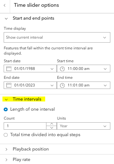
By default, three years of data will be displayed. You’ll need to change this: open the Time slider options from the three dots to the right of the time slider bar > open Time intervals > set the Length of one interval to ‘1 year’.
Alternatively, follow these steps to create a map using the Digital Atlas and then add the DEA Land Cover datasets (along with as any other datasets that are of interest).
How to add DEA Land Cover from the Digital Atlas of Australia to your own Esri environment
Add the layer to your map.
In the top menu bar, click File > Add Data > Add Data…
Select Add layer from URL then add one of the following URLs.
-
https://di-daa.img.arcgis.com/arcgis/rest/services/Land_and_vegetation/DEA_Landcover_Landsat_Level3/ImageServer
-
https://di-daa.img.arcgis.com/arcgis/rest/services/Land_and_vegetation/DEA_Landcover_Landsat_Level4/ImageServer
-
Note that the layer type is ArcGIS Server web service.
Click Add.
Set the time internal to ‘1 year’.
Ensure that the time slider is enabled to allow you to navigate through the annual layers in the dataset.
By default, three years of data will be displayed. You’ll need to change this: open the Time slider options from the three dots to the right of the time slider bar > open Time intervals > set the Length of one interval to ‘1 year’.
Learn more about how to add Esri web services to an ArcGIS environment.
Version history
Versions are numbered using the Semantic Versioning scheme (Major.Minor.Patch). Note that this list may include name changes and predecessor products.
v2.0.0 |
- |
Current version |
v1.0.0 |
of |
Changelog
30 Apr 2026: 2025 annual update now available
Digital Earth Australia (DEA) delivers refreshed 2025 annual data for a suite of terrestrial and inland water products, ensuring they reflect the most recent full calendar year of observations and remain consistent across the DEA product catalogue.
These updated datasets support consistent, year‑to‑year analysis of Australia’s land and inland water environments, helping users monitor change, compare trends over time, and apply the latest information with confidence.
By refreshing these products on an annual cycle, DEA continues to provide a nationally consistent foundation for land and water analysis, aligned across the broader DEA product catalogue.
29 Apr 2026: Patching of misclassified data
The tile x28y46 on the West Australian coast has been updated after a classification error was identified. Some areas of ocean in this tile were misclassified as mangroves and this has been corrected in the historical records.
10 Sep 2025: DEA Land Cover continental mosaics
We’ve added a new way to access our DEA Land Cover product; it is now available as continental mosaics, in Cloud-optimised GeoTIFF (COG) format. These mosaics provide a single-file representation of land cover data for each year available in the time series, removing the complexity of managing tiled datasets and making it easier to work with land cover data across Australia.
These COG mosaics are designed for fast and efficient streaming over the internet, loading only the portions of the file that are visible in your current view. This makes them ideal for use in GIS platforms such as QGIS and ESRI’s software, where users can interact with the DEA Land Cover dataset without needing to download entire files.
To enhance visualisation and interpretation, we also provide Virtual Raster (VRT) files with embedded colour styling aligned to the official DEA colour scheme. These VRTs make the data ready-to-use and visually meaningful out of the box.
The mosaics and VRTs can also be streamed for use in Python workflows using tools such as rioxarray.
Explore the latest year’s continental mosaics (2024)
Learn how to use DEA Land Cover continental mosaics
10 Sep 2025: DEA data in the Digital Atlas of Australia
The DEA Coastlines, DEA Mangroves, and DEA Water Observations Multi-Year Summary datasets have now been added to the Digital Atlas, joining DEA Land Cover. This integration marks a significant milestone in how DEA data can be accessed, visualised, and applied. By embedding DEA products into the Digital Atlas, users can now interact with trusted Earth observation datasets alongside other authoritative national data — unlocking powerful new opportunities for cross-sector analysis and decision-making.
June 2025: Resolved issue with missing data and artefacts in northern Western Australia
An issue was identified affecting data availability and causing classification artefacts across several tiles in northern Western Australia, particularly between 1988 and 2005. The primary affected tiles were x39y49, x40y47, and x41y45, although a total of 17 adjacent tiles (including the three mentioned) experienced the issue.
The root cause was traced to Geometric Quality Assessment (GQA) values falling below the acceptable threshold set. This threshold was used to filter out low-quality Landsat scenes from the Analysis Ready Data (ARD) inputs used to generate DEA Land Cover. The areas affected by this issue corresponded to regions where ground control points may shift over time, such as areas with shifting sand dunes, leading to inconsistencies in the orthorectification process. As a result, a large number of ARD scenes, not necessarily unusable, were excluded due to their lower GQA scores, reducing data coverage in the output product.
The issue was resolved by disabling GQA-based filtering in the affected areas, after observing that this had no noticeable impact on image sharpness or output quality.
Figure 1. Time series animation showing the frequency of missing data in the affected region. On the left is a true-colour time series of the yearly geomedian, for reference. On the right is a time series of the yearly clear observation count.
30 Apr 2025: The 2024 annual data is now available
You are now able to access the latest data via DEA Maps and other methods. View the Tech Alert.
Version 2.0.0
This latest version introduces improvements to the DEA Land Cover product, enhancing the translation of over three decades of satellite imagery into evidence of how Australia’s land, vegetation and waterbodies have changed over time.
Breaking change: Shift in grid origin point — The south-west origin point of the DEA Summary Product Grid has been shifted 18 tiles west and 15 tiles south. Therefore, all tile grid references have been changed. For instance, a tile reference of
x10y10has changed tox28y25.Breaking change: Data structure changes — Land Cover version 1.0 contained several TIF files including
waterstt-wat-cat-l4a.tif,watersea-veg-cat-l4a-au.tif,waterper-wat-cat-l4d-au.tif,lifeform-veg-cat-l4a.tif,inttidal-wat-cat-l4a.tif,canopyco-veg-cat-l4d.tif, andbaregrad-phy-cat-l4d-au.tif. These will not be provided in Land Cover 2.0 because the classifications are instead contained within thelevel4.tiffile, allowing users to filter the results as required. An RGB TIF colour representation of the Land Cover classifications is also no longer available. Instead, a style file will be provided that can be uploaded to your GIS software which will apply the same colour representations of the classifications in the Level 3 and Level 4 TIF files.Improved cloud masking to reduce noise — The masking of clouds and cloud shadows applied to DEA Land Cover model’s input data was improved, resulting in fewer noisy pixels in the final Land Cover product.
Landsat 9 included — Landsat 9 is included from 2022 onwards, leading to improved performance compared to the standalone Landsat 8 product. This is due to the increased number of observations from the combined Landsat 8 and 9 sensors.
Machine Learning Upgrade — The settings for machine learning (ML) methods and algorithms have been changed to improve performance. This is for woody cover, cultivated vegetation, and artificial surface classification. The Urban model uses a different ML approach, shifting from a pixel-based to a raster-based method, and a new model was trained using collection 3 data. The cultivated model maintains the same approach, but the input features were re-engineered using Geoscience Australia’s collection 3 data, and the model was re-trained. The woody cover model also follows the same approach, with the model being re-trained using Geoscience Australia’s collection 3 data.
Pixel resolution — The pixel resolution for Land Cover 2.0 has changed from 25m to 30m resolution.
Product ID Update — The Land Cover product ID has been updated to reflect the new ARD collection being used. It was changed to
ga_ls_landcover_class_cyear_3. This ID is used to load data from the Open Data Cube (ODC).‘No data’ value changed — The ‘no data’ value has been changed from ‘0’ to ‘255’ to be consistent with other DEA derivative products.
Level 4 classification update — The level 4 classifications have been updated to include the class ‘Cultivated Terrestrial Vegetated: Woody’.
Collection Upgrade — Land Cover version 2.0 is based on Geoscience Australia’s latest Landsat collection 3 analysis ready data.
Frequently Asked Questions
What are the differences between Version 1.0 and Version 2.0 of this product?
The main differences are as follows.
Version 1.0 (Collection 2) had a spatial resolution of 25 m, while Version 2.0 (Collection 3) has a spatial resolution of 30 m.
The ‘No data’ value has changed from ‘0’ to ‘255’. This is for consistency with other DEA derivative products.
The descriptor layers are now only accessible on DEA Maps. These layers aggregate information on specific categories such as the distinction between ‘Herbaceous’ and ‘Woody’ Natural Terrestrial Vegetation.
While the overall performance of Version 2.0 is similar to Version 1.0, the classification of Artificial Surface (AS) is notably better in Version 2.0, so the total number of pixels in that class is considerably higher. The Woody Cover ratio also seems to have improved in Version 2.0.
Some inconsistencies were observed in the areas assigned to the Cultivated Terrestrial Vegetation class between the two versions; however, the overall accuracy for this class remains similar between the two collections.
There is a notable increase in data affected by stripe artefacts from the Landsat 7 SLC-off failure from 2003 to 2011.
For more details, see the Quality tab.
What are the main limitations of the DEA Land Cover classification?
There are limitations originating from both the source satellite data and the algorithms applied to generate the final Land Cover product.
A fundamental limitation of any form of Earth Observation is data availability. Inconsistent data coverage and extended cloud cover periods can lead to gaps in the data, potentially missing entire intra-annual cycles, and this impairs the accuracy of the algorithm.
Another limitation arises from the spatial resolution of 30 m. Smaller landscape features could be missed entirely and incorrectly classified as the surrounding terrain.
Inaccuracies resulting from the performance of the algorithms generally occur when features within the satellite images resemble different features, leading to misclassification. Some examples are as follows: a) Events such as fires and rainfall can cause a response in vegetation that mirrors that of agricultural areas; b) Canopy in residential suburbs may obscure the correct identification of Artificial Surfaces; c) Shadows cast by buildings in dense urban areas can be classified as water; d) Bright sandy regions can be assigned to the Artificial Surfaces class.
Additionally, lack of training data for specific sub-classes and filters applied to the input images can limit the capabilities of the models to detect some environment types.
For more details, see the Quality tab.
What is the difference between Level 3 and Level 4 of the product?
DEA Land Cover is based on the globally applicable Food and Agriculture Organisation’s (FAO) Land Cover Classification System (LCCS). The Level 3 classifications are high-level macro-categories that broadly classify the continent into six classes.
The Level 4 classifications combine the Level 3 classes with their associated descriptors, resulting in more granular classes. For example, it differentiates between woody and herbaceous vegetation, as well as between open, closed, and sparse cover. It also provides information on water persistence, which corresponds to the number of months in a given year when water was present.
For more details, see the Quality tab.
Which Landsat satellites were used for generating the DEA Land Cover classification?
To generate the Land Cover classification for each calendar year, annual statistics (January to December) derived from the following Landsat satellites were used: Landsat 5, Landsat 7, Landsat 8, Landsat 9
This is an improvement over Version 1.0, which only used Landsat 5, Landsat 7, and Landsat 8.
For more details, see the Specifications tab and Quality tab.
Is this data available for free?
Yes, the DEA Land Cover data is free of charge and released under the Creative Commons Attribution 4.0 International Licence. However, licenses for specific platforms where the Land Cover data can be accessed, as well as additional data available on those platforms may vary.
For more details, see the Access tab and Credits tab.
Acknowledgments
DEA acknowledges the contribution of several collaborators who helped to create this Land Cover product.
CSIRO — Anna Richards, Becky Schmidt, Kristen Williams
UNSW — Graciela Metternicht
Department of Agriculture, Water and Environment — Jane Stewart, Lucy Randall, Lucy Gramenz
ANU — Albert van Dijk
Tasmania DPIPWE — Lindsay Mitchell
License and copyright
© Commonwealth of Australia (Geoscience Australia).
Released under Creative Commons Attribution 4.0 International Licence.