Exporting data to NetCDF files

• Sign up to the DEA Sandbox to run this notebook interactively from a browser

• Compatibility: Notebook currently compatible with both the NCI and DEA Sandbox environments

• Products used: ga_ls8cls9c_gm_cyear_3

Background

NetCDF is a file format for storing multidimensional scientific data. This file format supports datasets containing multiple observation dates, as well as multiple bands. It is a native format for storing the xarray datasets that are produced by Open Data Cube, i.e. by dc.load commands.

NetCDF files should follow Climate and Forecast (CF) metadata conventions for the description of Earth sciences data. By providing metadata such as geospatial coordinates and sensor information in the same file as the data, CF conventions allow NetCDF files to be “self-describing”. This makes CF-compliant NetCDFs a useful way to save multidimensional data loaded from Digital Earth Australia, as the data can later be loaded with all the information required for further analysis.

The xarray library which underlies the Open Data Cube (and hence Digital Earth Australia) was specifically designed for representing NetCDF files in Python. However, some geospatial metadata is represented quite differently between the NetCDF-CF conventions versus the GDAL (or proj4) model that is common to most geospatial software (including ODC, e.g. for reprojecting raster data when necessary). The main difference between to_netcdf (in xarray natively) and write_dataset_to_netcdf (provided by datacube) is that the latter is able to appropriately serialise the coordinate reference system object which is associated to the dataset.

Description

In this notebook we will load some data from Digital Earth Australia and then write it to a (CF-compliant) NetCDF file using the write_dataset_to_netcdf function provided by datacube. We will then verify the file was saved correctly, and (optionally) clean up.

---

Getting started

To run this analysis, run all the cells in the notebook, starting with the “Load packages” cell.

Load packages

%matplotlib inline

import datacube
import xarray as xr
from datacube.drivers.netcdf import write_dataset_to_netcdf

Connect to the datacube

dc = datacube.Datacube(app='Exporting_NetCDFs')

Load data from the datacube

Here we load a sample dataset from the DEA Landsat-8 Annual Geomedian product (ga_ls8c_nbart_gm_cyear_3). The loaded data is multidimensional, and contains two time-steps (2015, 2016) and six satellite bands (blue, green, red, nir, swir1, swir2).

lat, lon = -35.282052, 149.128667  # City Hill, Canberra
buffer = 0.01  # Approx. 1km

# Load data from the datacube
ds = dc.load(product='ga_ls8cls9c_gm_cyear_3',
             lat=(lat - buffer, lat + buffer),
             lon=(lon - buffer, lon + buffer),
             time=('2015', '2016'))

# Print output data
ds

<xarray.Dataset> Size: 304kB
Dimensions:       (time: 2, y: 82, x: 71)
Coordinates:
  * time          (time) datetime64[ns] 16B 2015-07-02T11:59:59.999999 2016-0...
  * y             (y) float64 656B -3.956e+06 -3.956e+06 ... -3.959e+06
  * x             (x) float64 568B 1.549e+06 1.549e+06 ... 1.551e+06 1.551e+06
    spatial_ref   int32 4B 3577
Data variables:
    nbart_blue    (time, y, x) int16 23kB 646 652 693 686 ... 519 558 534 425
    nbart_green   (time, y, x) int16 23kB 838 843 962 945 ... 770 794 779 641
    nbart_red     (time, y, x) int16 23kB 910 999 1183 1157 ... 828 856 812 636
    nbart_nir     (time, y, x) int16 23kB 1939 2016 2134 2349 ... 2607 2676 2619
    nbart_swir_1  (time, y, x) int16 23kB 1825 2052 2318 2395 ... 1998 2049 1795
    nbart_swir_2  (time, y, x) int16 23kB 1450 1632 1933 1924 ... 1276 1266 1050
    sdev          (time, y, x) float32 47kB 0.001365 0.001093 ... 0.007874
    edev          (time, y, x) float32 47kB 446.6 572.6 674.6 ... 529.2 521.8
    bcdev         (time, y, x) float32 47kB 0.06709 0.06056 ... 0.07159 0.07628
    count         (time, y, x) int16 23kB 23 23 23 23 23 23 ... 15 16 16 17 17
Attributes:
    crs:           epsg:3577
    grid_mapping:  spatial_ref

xarray.Dataset

• Dimensions:
  • time: 2
  • y: 82
  • x: 71
• Coordinates: (4)
  • time
    (time)
    datetime64[ns]
    2015-07-02T11:59:59.999999 2016-...

    units :

    seconds since 1970-01-01 00:00:00

    array(['2015-07-02T11:59:59.999999000', '2016-07-01T23:59:59.999999000'],
          dtype='datetime64[ns]')

  • y
    (y)
    float64
    -3.956e+06 ... -3.959e+06

    units :

    metre

    resolution :

    -30.0

    crs :

    epsg:3577

    array([-3956355., -3956385., -3956415., -3956445., -3956475., -3956505.,
           -3956535., -3956565., -3956595., -3956625., -3956655., -3956685.,
           -3956715., -3956745., -3956775., -3956805., -3956835., -3956865.,
           -3956895., -3956925., -3956955., -3956985., -3957015., -3957045.,
           -3957075., -3957105., -3957135., -3957165., -3957195., -3957225.,
           -3957255., -3957285., -3957315., -3957345., -3957375., -3957405.,
           -3957435., -3957465., -3957495., -3957525., -3957555., -3957585.,
           -3957615., -3957645., -3957675., -3957705., -3957735., -3957765.,
           -3957795., -3957825., -3957855., -3957885., -3957915., -3957945.,
           -3957975., -3958005., -3958035., -3958065., -3958095., -3958125.,
           -3958155., -3958185., -3958215., -3958245., -3958275., -3958305.,
           -3958335., -3958365., -3958395., -3958425., -3958455., -3958485.,
           -3958515., -3958545., -3958575., -3958605., -3958635., -3958665.,
           -3958695., -3958725., -3958755., -3958785.])

  • x
    (x)
    float64
    1.549e+06 1.549e+06 ... 1.551e+06

    units :

    metre

    resolution :

    30.0

    crs :

    epsg:3577

    array([1549365., 1549395., 1549425., 1549455., 1549485., 1549515., 1549545.,
           1549575., 1549605., 1549635., 1549665., 1549695., 1549725., 1549755.,
           1549785., 1549815., 1549845., 1549875., 1549905., 1549935., 1549965.,
           1549995., 1550025., 1550055., 1550085., 1550115., 1550145., 1550175.,
           1550205., 1550235., 1550265., 1550295., 1550325., 1550355., 1550385.,
           1550415., 1550445., 1550475., 1550505., 1550535., 1550565., 1550595.,
           1550625., 1550655., 1550685., 1550715., 1550745., 1550775., 1550805.,
           1550835., 1550865., 1550895., 1550925., 1550955., 1550985., 1551015.,
           1551045., 1551075., 1551105., 1551135., 1551165., 1551195., 1551225.,
           1551255., 1551285., 1551315., 1551345., 1551375., 1551405., 1551435.,
           1551465.])

  • spatial_ref
    ()
    int32
    3577

    spatial_ref :

    PROJCS["GDA94 / Australian Albers",GEOGCS["GDA94",DATUM["Geocentric_Datum_of_Australia_1994",SPHEROID["GRS 1980",6378137,298.257222101,AUTHORITY["EPSG","7019"]],AUTHORITY["EPSG","6283"]],PRIMEM["Greenwich",0,AUTHORITY["EPSG","8901"]],UNIT["degree",0.0174532925199433,AUTHORITY["EPSG","9122"]],AUTHORITY["EPSG","4283"]],PROJECTION["Albers_Conic_Equal_Area"],PARAMETER["latitude_of_center",0],PARAMETER["longitude_of_center",132],PARAMETER["standard_parallel_1",-18],PARAMETER["standard_parallel_2",-36],PARAMETER["false_easting",0],PARAMETER["false_northing",0],UNIT["metre",1,AUTHORITY["EPSG","9001"]],AXIS["Easting",EAST],AXIS["Northing",NORTH],AUTHORITY["EPSG","3577"]]

    grid_mapping_name :

    albers_conical_equal_area

    array(3577, dtype=int32)

• Data variables: (10)
  • nbart_blue
    (time, y, x)
    int16
    646 652 693 686 ... 519 558 534 425

    units :

    1

    nodata :

    -999

    crs :

    epsg:3577

    grid_mapping :

    spatial_ref

    array([[[ 646,  652,  693, ...,  254,  269,  300],
            [ 884, 1188,  991, ...,  313,  347,  338],
            [1681, 1234,  733, ...,  368,  413,  411],
            ...,
            [ 432,  491,  449, ...,  363,  321,  467],
            [ 351,  468,  494, ...,  496,  444,  355],
            [ 310,  341,  484, ...,  554,  565,  441]],
    
           [[ 694,  703,  834, ...,  266,  281,  299],
            [ 929, 1205, 1076, ...,  312,  359,  345],
            [1700, 1226,  763, ...,  366,  405,  406],
            ...,
            [ 412,  494,  496, ...,  364,  338,  491],
            [ 376,  465,  432, ...,  479,  437,  362],
            [ 284,  322,  363, ...,  558,  534,  425]]], dtype=int16)

  • nbart_green
    (time, y, x)
    int16
    838 843 962 945 ... 770 794 779 641

    units :

    1

    nodata :

    -999

    crs :

    epsg:3577

    grid_mapping :

    spatial_ref

    array([[[ 838,  843,  962, ...,  410,  434,  477],
            [1032, 1397, 1288, ...,  479,  519,  513],
            [1980, 1473,  938, ...,  548,  617,  599],
            ...,
            [ 631,  720,  689, ...,  491,  438,  575],
            [ 530,  677,  705, ...,  686,  646,  512],
            [ 454,  493,  664, ...,  795,  821,  660]],
    
           [[ 916,  908, 1128, ...,  445,  470,  487],
            [1114, 1425, 1379, ...,  501,  550,  534],
            [1994, 1463,  995, ...,  564,  628,  615],
            ...,
            [ 598,  714,  733, ...,  506,  468,  610],
            [ 545,  678,  613, ...,  681,  640,  526],
            [ 412,  463,  513, ...,  794,  779,  641]]], dtype=int16)

  • nbart_red
    (time, y, x)
    int16
    910 999 1183 1157 ... 856 812 636

    units :

    1

    nodata :

    -999

    crs :

    epsg:3577

    grid_mapping :

    spatial_ref

    array([[[ 910,  999, 1183, ...,  358,  380,  427],
            [1158, 1544, 1436, ...,  439,  502,  496],
            [1967, 1528,  997, ...,  594,  778,  734],
            ...,
            [ 626,  731,  729, ...,  524,  444,  594],
            [ 516,  707,  718, ...,  763,  674,  513],
            [ 433,  485,  665, ...,  845,  868,  664]],
    
           [[1001, 1095, 1395, ...,  376,  397,  425],
            [1213, 1577, 1569, ...,  441,  514,  498],
            [1967, 1498, 1034, ...,  590,  762,  712],
            ...,
            [ 598,  754,  800, ...,  530,  476,  609],
            [ 558,  711,  598, ...,  753,  670,  525],
            [ 374,  441,  471, ...,  856,  812,  636]]], dtype=int16)

  • nbart_nir
    (time, y, x)
    int16
    1939 2016 2134 ... 2607 2676 2619

    units :

    1

    nodata :

    -999

    crs :

    epsg:3577

    grid_mapping :

    spatial_ref

    array([[[1939, 2016, 2134, ..., 2008, 2007, 2103],
            [1971, 2170, 2165, ..., 2002, 1943, 2004],
            [2679, 2249, 1970, ..., 2242, 2221, 2160],
            ...,
            [2359, 2574, 2752, ..., 1863, 2003, 1646],
            [1690, 2428, 2402, ..., 2185, 2427, 2237],
            [ 695, 1572, 2330, ..., 2580, 2631, 2633]],
    
           [[2139, 2217, 2392, ..., 2239, 2242, 2252],
            [2214, 2399, 2528, ..., 2236, 2176, 2200],
            [3019, 2688, 2492, ..., 2441, 2422, 2424],
            ...,
            [2500, 2716, 2790, ..., 2029, 2093, 1727],
            [1724, 2540, 2708, ..., 2293, 2503, 2289],
            [ 652, 1652, 2681, ..., 2607, 2676, 2619]]], dtype=int16)

  • nbart_swir_1
    (time, y, x)
    int16
    1825 2052 2318 ... 1998 2049 1795

    units :

    1

    nodata :

    -999

    crs :

    epsg:3577

    grid_mapping :

    spatial_ref

    array([[[1825, 2052, 2318, ..., 1080, 1110, 1259],
            [2080, 2582, 2339, ..., 1244, 1291, 1346],
            [2768, 2370, 1778, ..., 1669, 2032, 2060],
            ...,
            [1647, 1951, 1969, ..., 1232, 1088, 1091],
            [1186, 1851, 1785, ..., 1757, 1733, 1369],
            [ 452, 1006, 1600, ..., 1971, 2080, 1778]],
    
           [[2062, 2314, 2744, ..., 1232, 1254, 1313],
            [2292, 2751, 2609, ..., 1322, 1369, 1402],
            [2972, 2503, 1900, ..., 1724, 2055, 2065],
            ...,
            [1622, 2012, 2166, ..., 1340, 1243, 1194],
            [1281, 1885, 1701, ..., 1793, 1797, 1502],
            [ 474,  995, 1384, ..., 1998, 2049, 1795]]], dtype=int16)

  • nbart_swir_2
    (time, y, x)
    int16
    1450 1632 1933 ... 1276 1266 1050

    units :

    1

    nodata :

    -999

    crs :

    epsg:3577

    grid_mapping :

    spatial_ref

    array([[[1450, 1632, 1933, ...,  595,  627,  724],
            [1843, 2393, 1968, ...,  766,  856,  895],
            [2330, 2013, 1353, ..., 1204, 1633, 1550],
            ...,
            [1004, 1224, 1179, ...,  764,  639,  707],
            [ 696, 1145, 1146, ..., 1161, 1061,  810],
            [ 283,  622, 1030, ..., 1276, 1319, 1057]],
    
           [[1584, 1834, 2273, ...,  668,  687,  734],
            [2050, 2516, 2178, ...,  791,  881,  902],
            [2497, 2110, 1392, ..., 1228, 1600, 1539],
            ...,
            [ 954, 1235, 1286, ...,  800,  718,  785],
            [ 753, 1114,  979, ..., 1140, 1078,  882],
            [ 306,  572,  749, ..., 1276, 1266, 1050]]], dtype=int16)

  • sdev
    (time, y, x)
    float32
    0.001365 0.001093 ... 0.007874

    units :

    1

    nodata :

    nan

    crs :

    epsg:3577

    grid_mapping :

    spatial_ref

    array([[[0.00136494, 0.00109345, 0.00102232, ..., 0.0035431 ,
             0.00225836, 0.00131013],
            [0.00232193, 0.00200628, 0.00065535, ..., 0.00128055,
             0.00093364, 0.00051876],
            [0.00346745, 0.00227436, 0.0009675 , ..., 0.00111458,
             0.00108562, 0.00068424],
            ...,
            [0.00169171, 0.00128121, 0.0011914 , ..., 0.00629258,
             0.00675577, 0.00424329],
            [0.00089482, 0.00131263, 0.00398641, ..., 0.0031522 ,
             0.0059753 , 0.00848498],
            [0.00705463, 0.00343207, 0.01127079, ..., 0.00181916,
             0.00452003, 0.00408413]],
    
           [[0.00057813, 0.00067988, 0.00051909, ..., 0.00169298,
             0.0011502 , 0.00127093],
            [0.00198017, 0.00166392, 0.00056966, ..., 0.00065255,
             0.0004746 , 0.00076431],
            [0.00165381, 0.00277247, 0.00177942, ..., 0.00042058,
             0.00092927, 0.00070568],
            ...,
            [0.00132421, 0.0016675 , 0.00131503, ..., 0.00377701,
             0.00364647, 0.00193904],
            [0.00342573, 0.00281651, 0.00116335, ..., 0.00420736,
             0.00755949, 0.00462576],
            [0.0095879 , 0.00310031, 0.0011499 , ..., 0.00468731,
             0.00879017, 0.00787434]]], dtype=float32)

  • edev
    (time, y, x)
    float32
    446.6 572.6 674.6 ... 529.2 521.8

    units :

    1

    nodata :

    nan

    crs :

    epsg:3577

    grid_mapping :

    spatial_ref

    array([[[446.629  , 572.6432 , 674.57245, ..., 480.56732, 437.32538,
             378.33087],
            [521.99023, 644.199  , 621.86615, ..., 426.88974, 428.81622,
             354.3248 ],
            [723.7972 , 615.2347 , 610.9775 , ..., 351.10965, 384.44327,
             439.80612],
            ...,
            [267.96722, 303.1758 , 303.4271 , ..., 549.69104, 456.3231 ,
             424.81198],
            [186.02565, 258.1284 , 352.984  , ..., 439.81412, 627.8081 ,
             561.7128 ],
            [203.01413, 258.85754, 484.30222, ..., 360.07672, 495.64667,
             457.6419 ]],
    
           [[394.18707, 229.17564, 387.4192 , ..., 236.65935, 242.83882,
             240.7799 ],
            [471.3211 , 414.4274 , 388.27103, ..., 276.64944, 260.3425 ,
             264.67758],
            [443.58707, 545.663  , 421.6372 , ..., 177.92012, 250.03333,
             245.3816 ],
            ...,
            [219.5482 , 256.5675 , 420.37616, ..., 331.66434, 374.6099 ,
             379.96677],
            [321.92114, 394.3938 , 254.32779, ..., 330.87234, 490.41745,
             394.9598 ],
            [256.12473, 326.09033, 273.66736, ..., 380.99014, 529.1909 ,
             521.757  ]]], dtype=float32)

  • bcdev
    (time, y, x)
    float32
    0.06709 0.06056 ... 0.07159 0.07628

    units :

    1

    nodata :

    nan

    crs :

    epsg:3577

    grid_mapping :

    spatial_ref

    array([[[0.06709041, 0.0605608 , 0.07072702, ..., 0.0933525 ,
             0.08764967, 0.06833728],
            [0.06237958, 0.04724619, 0.06384891, ..., 0.0700784 ,
             0.07123768, 0.05785638],
            [0.05393218, 0.05209725, 0.0715287 , ..., 0.0449685 ,
             0.0400061 , 0.05624654],
            ...,
            [0.04002201, 0.03462613, 0.03393445, ..., 0.10367979,
             0.09910299, 0.08621374],
            [0.03512923, 0.03571169, 0.04966618, ..., 0.06871749,
             0.08630868, 0.10230352],
            [0.07850705, 0.0549629 , 0.07418688, ..., 0.04639209,
             0.06528548, 0.06504922]],
    
           [[0.05400456, 0.02466987, 0.03517222, ..., 0.04561653,
             0.04254045, 0.03686429],
            [0.04055117, 0.03317668, 0.03368507, ..., 0.04105748,
             0.03863918, 0.03539402],
            [0.03054159, 0.04177932, 0.04839323, ..., 0.02378825,
             0.03126076, 0.03141721],
            ...,
            [0.02673032, 0.03026228, 0.05133855, ..., 0.05916167,
             0.06358832, 0.06339435],
            [0.06011786, 0.05505569, 0.03900049, ..., 0.04814196,
             0.07211108, 0.05878207],
            [0.09429356, 0.06988396, 0.0433208 , ..., 0.04808231,
             0.07159099, 0.07627717]]], dtype=float32)

  • count
    (time, y, x)
    int16
    23 23 23 23 23 ... 15 16 16 17 17

    units :

    1

    nodata :

    -999

    crs :

    epsg:3577

    grid_mapping :

    spatial_ref

    array([[[23, 23, 23, ..., 24, 24, 24],
            [23, 23, 23, ..., 24, 24, 24],
            [23, 23, 23, ..., 24, 24, 24],
            ...,
            [20, 20, 21, ..., 20, 20, 20],
            [20, 20, 21, ..., 21, 20, 20],
            [20, 20, 21, ..., 19, 20, 20]],
    
           [[17, 17, 18, ..., 20, 20, 20],
            [17, 17, 17, ..., 20, 20, 20],
            [17, 17, 17, ..., 20, 20, 20],
            ...,
            [19, 19, 19, ..., 17, 18, 18],
            [19, 19, 19, ..., 16, 17, 16],
            [19, 19, 19, ..., 16, 17, 17]]], dtype=int16)

• Indexes: (3)
  • time
    PandasIndex

    PandasIndex(DatetimeIndex(['2015-07-02 11:59:59.999999', '2016-07-01 23:59:59.999999'], dtype='datetime64[ns]', name='time', freq=None))

  • y
    PandasIndex

    PandasIndex(Index([-3956355.0, -3956385.0, -3956415.0, -3956445.0, -3956475.0, -3956505.0,
           -3956535.0, -3956565.0, -3956595.0, -3956625.0, -3956655.0, -3956685.0,
           -3956715.0, -3956745.0, -3956775.0, -3956805.0, -3956835.0, -3956865.0,
           -3956895.0, -3956925.0, -3956955.0, -3956985.0, -3957015.0, -3957045.0,
           -3957075.0, -3957105.0, -3957135.0, -3957165.0, -3957195.0, -3957225.0,
           -3957255.0, -3957285.0, -3957315.0, -3957345.0, -3957375.0, -3957405.0,
           -3957435.0, -3957465.0, -3957495.0, -3957525.0, -3957555.0, -3957585.0,
           -3957615.0, -3957645.0, -3957675.0, -3957705.0, -3957735.0, -3957765.0,
           -3957795.0, -3957825.0, -3957855.0, -3957885.0, -3957915.0, -3957945.0,
           -3957975.0, -3958005.0, -3958035.0, -3958065.0, -3958095.0, -3958125.0,
           -3958155.0, -3958185.0, -3958215.0, -3958245.0, -3958275.0, -3958305.0,
           -3958335.0, -3958365.0, -3958395.0, -3958425.0, -3958455.0, -3958485.0,
           -3958515.0, -3958545.0, -3958575.0, -3958605.0, -3958635.0, -3958665.0,
           -3958695.0, -3958725.0, -3958755.0, -3958785.0],
          dtype='float64', name='y'))

  • x
    PandasIndex

    PandasIndex(Index([1549365.0, 1549395.0, 1549425.0, 1549455.0, 1549485.0, 1549515.0,
           1549545.0, 1549575.0, 1549605.0, 1549635.0, 1549665.0, 1549695.0,
           1549725.0, 1549755.0, 1549785.0, 1549815.0, 1549845.0, 1549875.0,
           1549905.0, 1549935.0, 1549965.0, 1549995.0, 1550025.0, 1550055.0,
           1550085.0, 1550115.0, 1550145.0, 1550175.0, 1550205.0, 1550235.0,
           1550265.0, 1550295.0, 1550325.0, 1550355.0, 1550385.0, 1550415.0,
           1550445.0, 1550475.0, 1550505.0, 1550535.0, 1550565.0, 1550595.0,
           1550625.0, 1550655.0, 1550685.0, 1550715.0, 1550745.0, 1550775.0,
           1550805.0, 1550835.0, 1550865.0, 1550895.0, 1550925.0, 1550955.0,
           1550985.0, 1551015.0, 1551045.0, 1551075.0, 1551105.0, 1551135.0,
           1551165.0, 1551195.0, 1551225.0, 1551255.0, 1551285.0, 1551315.0,
           1551345.0, 1551375.0, 1551405.0, 1551435.0, 1551465.0],
          dtype='float64', name='x'))

• Attributes: (2)

  crs :

  epsg:3577

  grid_mapping :

  spatial_ref

Export to a NetCDF file

To export a CF-compliant NetCDF file, we use the write_dataset_to_netcdf function:

write_dataset_to_netcdf(ds, 'output_netcdf.nc')

That’s all. The file has now been produced, and stored in the current working directory.

Reading back from saved NetCDF

Let’s start just by confirming the file now exists. We can use the special ! command to run command line tools directly within a Jupyter notebook. In the example below, ! ls *.nc runs the ls shell command, which will give us a list of any files in the NetCDF file format (i.e. with file names ending with .nc).

For an introduction to using shell commands in Jupyter, see the guide here.

! ls *.nc

output_netcdf.nc

We could inspect this file using external utilities such as gdalinfo or ncdump, or open it for visualisation e.g. in QGIS.

We can also load the file back into Python using xarray:

# Load the NetCDF from file
reloaded_ds = xr.open_dataset('output_netcdf.nc')

# Print loaded data
reloaded_ds

<xarray.Dataset> Size: 467kB
Dimensions:       (time: 2, y: 82, x: 71)
Coordinates:
  * time          (time) datetime64[ns] 16B 2015-07-02T11:59:59 2016-07-01T23...
  * y             (y) float64 656B -3.956e+06 -3.956e+06 ... -3.959e+06
  * x             (x) float64 568B 1.549e+06 1.549e+06 ... 1.551e+06 1.551e+06
    spatial_ref   int32 4B ...
Data variables:
    nbart_blue    (time, y, x) float32 47kB ...
    nbart_green   (time, y, x) float32 47kB ...
    nbart_red     (time, y, x) float32 47kB ...
    nbart_nir     (time, y, x) float32 47kB ...
    nbart_swir_1  (time, y, x) float32 47kB ...
    nbart_swir_2  (time, y, x) float32 47kB ...
    sdev          (time, y, x) float32 47kB ...
    edev          (time, y, x) float32 47kB ...
    bcdev         (time, y, x) float32 47kB ...
    count         (time, y, x) float32 47kB ...
Attributes:
    date_created:           2024-06-17T06:29:45.296627
    Conventions:            CF-1.6, ACDD-1.3
    history:                NetCDF-CF file created by datacube version '1.8.1...
    geospatial_bounds:      POLYGON ((149.11516275211676 -35.272298024386345,...
    geospatial_bounds_crs:  EPSG:4326
    geospatial_lat_min:     -35.29422745554414
    geospatial_lat_max:     -35.269737305748244
    geospatial_lat_units:   degrees_north
    geospatial_lon_min:     149.11516275211676
    geospatial_lon_max:     149.14203545880687
    geospatial_lon_units:   degrees_east

xarray.Dataset

• Dimensions:
  • time: 2
  • y: 82
  • x: 71
• Coordinates: (4)
  • time
    (time)
    datetime64[ns]
    2015-07-02T11:59:59 2016-07-01T2...

    standard_name :

    time

    long_name :

    Time, unix time-stamp

    axis :

    T

    array(['2015-07-02T11:59:59.000000000', '2016-07-01T23:59:59.000000000'],
          dtype='datetime64[ns]')

  • y
    (y)
    float64
    -3.956e+06 ... -3.959e+06

    units :

    metre

    standard_name :

    projection_y_coordinate

    long_name :

    y coordinate of projection

    array([-3956355., -3956385., -3956415., -3956445., -3956475., -3956505.,
           -3956535., -3956565., -3956595., -3956625., -3956655., -3956685.,
           -3956715., -3956745., -3956775., -3956805., -3956835., -3956865.,
           -3956895., -3956925., -3956955., -3956985., -3957015., -3957045.,
           -3957075., -3957105., -3957135., -3957165., -3957195., -3957225.,
           -3957255., -3957285., -3957315., -3957345., -3957375., -3957405.,
           -3957435., -3957465., -3957495., -3957525., -3957555., -3957585.,
           -3957615., -3957645., -3957675., -3957705., -3957735., -3957765.,
           -3957795., -3957825., -3957855., -3957885., -3957915., -3957945.,
           -3957975., -3958005., -3958035., -3958065., -3958095., -3958125.,
           -3958155., -3958185., -3958215., -3958245., -3958275., -3958305.,
           -3958335., -3958365., -3958395., -3958425., -3958455., -3958485.,
           -3958515., -3958545., -3958575., -3958605., -3958635., -3958665.,
           -3958695., -3958725., -3958755., -3958785.])

  • x
    (x)
    float64
    1.549e+06 1.549e+06 ... 1.551e+06

    units :

    metre

    standard_name :

    projection_x_coordinate

    long_name :

    x coordinate of projection

    array([1549365., 1549395., 1549425., 1549455., 1549485., 1549515., 1549545.,
           1549575., 1549605., 1549635., 1549665., 1549695., 1549725., 1549755.,
           1549785., 1549815., 1549845., 1549875., 1549905., 1549935., 1549965.,
           1549995., 1550025., 1550055., 1550085., 1550115., 1550145., 1550175.,
           1550205., 1550235., 1550265., 1550295., 1550325., 1550355., 1550385.,
           1550415., 1550445., 1550475., 1550505., 1550535., 1550565., 1550595.,
           1550625., 1550655., 1550685., 1550715., 1550745., 1550775., 1550805.,
           1550835., 1550865., 1550895., 1550925., 1550955., 1550985., 1551015.,
           1551045., 1551075., 1551105., 1551135., 1551165., 1551195., 1551225.,
           1551255., 1551285., 1551315., 1551345., 1551375., 1551405., 1551435.,
           1551465.])

  • spatial_ref
    ()
    int32
    ...

    grid_mapping_name :

    albers_conical_equal_area

    standard_parallel :

    [-18. -36.]

    longitude_of_central_meridian :

    132.0

    latitude_of_projection_origin :

    0.0

    false_easting :

    0.0

    false_northing :

    0.0

    long_name :

    GDA94 / Australian Albers

    semi_major_axis :

    6378137.0

    semi_minor_axis :

    6356752.314140356

    inverse_flattening :

    298.257222101

    crs_wkt :

    PROJCS["GDA94 / Australian Albers",GEOGCS["GDA94",DATUM["Geocentric_Datum_of_Australia_1994",SPHEROID["GRS 1980",6378137,298.257222101,AUTHORITY["EPSG","7019"]],AUTHORITY["EPSG","6283"]],PRIMEM["Greenwich",0,AUTHORITY["EPSG","8901"]],UNIT["degree",0.0174532925199433,AUTHORITY["EPSG","9122"]],AUTHORITY["EPSG","4283"]],PROJECTION["Albers_Conic_Equal_Area"],PARAMETER["latitude_of_center",0],PARAMETER["longitude_of_center",132],PARAMETER["standard_parallel_1",-18],PARAMETER["standard_parallel_2",-36],PARAMETER["false_easting",0],PARAMETER["false_northing",0],UNIT["metre",1,AUTHORITY["EPSG","9001"]],AXIS["Easting",EAST],AXIS["Northing",NORTH],AUTHORITY["EPSG","3577"]]

    spatial_ref :

    PROJCS["GDA94 / Australian Albers",GEOGCS["GDA94",DATUM["Geocentric_Datum_of_Australia_1994",SPHEROID["GRS 1980",6378137,298.257222101,AUTHORITY["EPSG","7019"]],AUTHORITY["EPSG","6283"]],PRIMEM["Greenwich",0,AUTHORITY["EPSG","8901"]],UNIT["degree",0.0174532925199433,AUTHORITY["EPSG","9122"]],AUTHORITY["EPSG","4283"]],PROJECTION["Albers_Conic_Equal_Area"],PARAMETER["latitude_of_center",0],PARAMETER["longitude_of_center",132],PARAMETER["standard_parallel_1",-18],PARAMETER["standard_parallel_2",-36],PARAMETER["false_easting",0],PARAMETER["false_northing",0],UNIT["metre",1,AUTHORITY["EPSG","9001"]],AXIS["Easting",EAST],AXIS["Northing",NORTH],AUTHORITY["EPSG","3577"]]

    GeoTransform :

    [ 1.54935e+06 3.00000e+01 0.00000e+00 -3.95634e+06 0.00000e+00 -3.00000e+01]

    [1 values with dtype=int32]

• Data variables: (10)
  • nbart_blue
    (time, y, x)
    float32
    ...

    grid_mapping :

    spatial_ref

    units :

    1

    [11644 values with dtype=float32]

  • nbart_green
    (time, y, x)
    float32
    ...

    grid_mapping :

    spatial_ref

    units :

    1

    [11644 values with dtype=float32]

  • nbart_red
    (time, y, x)
    float32
    ...

    grid_mapping :

    spatial_ref

    units :

    1

    [11644 values with dtype=float32]

  • nbart_nir
    (time, y, x)
    float32
    ...

    grid_mapping :

    spatial_ref

    units :

    1

    [11644 values with dtype=float32]

  • nbart_swir_1
    (time, y, x)
    float32
    ...

    grid_mapping :

    spatial_ref

    units :

    1

    [11644 values with dtype=float32]

  • nbart_swir_2
    (time, y, x)
    float32
    ...

    grid_mapping :

    spatial_ref

    units :

    1

    [11644 values with dtype=float32]

  • sdev
    (time, y, x)
    float32
    ...

    grid_mapping :

    spatial_ref

    units :

    1

    [11644 values with dtype=float32]

  • edev
    (time, y, x)
    float32
    ...

    grid_mapping :

    spatial_ref

    units :

    1

    [11644 values with dtype=float32]

  • bcdev
    (time, y, x)
    float32
    ...

    grid_mapping :

    spatial_ref

    units :

    1

    [11644 values with dtype=float32]

  • count
    (time, y, x)
    float32
    ...

    grid_mapping :

    spatial_ref

    units :

    1

    [11644 values with dtype=float32]

• Indexes: (3)
  • time
    PandasIndex

    PandasIndex(DatetimeIndex(['2015-07-02 11:59:59', '2016-07-01 23:59:59'], dtype='datetime64[ns]', name='time', freq=None))

  • y
    PandasIndex

    PandasIndex(Index([-3956355.0, -3956385.0, -3956415.0, -3956445.0, -3956475.0, -3956505.0,
           -3956535.0, -3956565.0, -3956595.0, -3956625.0, -3956655.0, -3956685.0,
           -3956715.0, -3956745.0, -3956775.0, -3956805.0, -3956835.0, -3956865.0,
           -3956895.0, -3956925.0, -3956955.0, -3956985.0, -3957015.0, -3957045.0,
           -3957075.0, -3957105.0, -3957135.0, -3957165.0, -3957195.0, -3957225.0,
           -3957255.0, -3957285.0, -3957315.0, -3957345.0, -3957375.0, -3957405.0,
           -3957435.0, -3957465.0, -3957495.0, -3957525.0, -3957555.0, -3957585.0,
           -3957615.0, -3957645.0, -3957675.0, -3957705.0, -3957735.0, -3957765.0,
           -3957795.0, -3957825.0, -3957855.0, -3957885.0, -3957915.0, -3957945.0,
           -3957975.0, -3958005.0, -3958035.0, -3958065.0, -3958095.0, -3958125.0,
           -3958155.0, -3958185.0, -3958215.0, -3958245.0, -3958275.0, -3958305.0,
           -3958335.0, -3958365.0, -3958395.0, -3958425.0, -3958455.0, -3958485.0,
           -3958515.0, -3958545.0, -3958575.0, -3958605.0, -3958635.0, -3958665.0,
           -3958695.0, -3958725.0, -3958755.0, -3958785.0],
          dtype='float64', name='y'))

  • x
    PandasIndex

    PandasIndex(Index([1549365.0, 1549395.0, 1549425.0, 1549455.0, 1549485.0, 1549515.0,
           1549545.0, 1549575.0, 1549605.0, 1549635.0, 1549665.0, 1549695.0,
           1549725.0, 1549755.0, 1549785.0, 1549815.0, 1549845.0, 1549875.0,
           1549905.0, 1549935.0, 1549965.0, 1549995.0, 1550025.0, 1550055.0,
           1550085.0, 1550115.0, 1550145.0, 1550175.0, 1550205.0, 1550235.0,
           1550265.0, 1550295.0, 1550325.0, 1550355.0, 1550385.0, 1550415.0,
           1550445.0, 1550475.0, 1550505.0, 1550535.0, 1550565.0, 1550595.0,
           1550625.0, 1550655.0, 1550685.0, 1550715.0, 1550745.0, 1550775.0,
           1550805.0, 1550835.0, 1550865.0, 1550895.0, 1550925.0, 1550955.0,
           1550985.0, 1551015.0, 1551045.0, 1551075.0, 1551105.0, 1551135.0,
           1551165.0, 1551195.0, 1551225.0, 1551255.0, 1551285.0, 1551315.0,
           1551345.0, 1551375.0, 1551405.0, 1551435.0, 1551465.0],
          dtype='float64', name='x'))

• Attributes: (11)

  date_created :

  2024-06-17T06:29:45.296627

  Conventions :

  CF-1.6, ACDD-1.3

  history :

  NetCDF-CF file created by datacube version '1.8.18' at 20240617.

  geospatial_bounds :

  POLYGON ((149.11516275211676 -35.272298024386345, 149.11878233641355 -35.29422745554414, 149.14203545880687 -35.2916660557473, 149.13841107635864 -35.269737305748244, 149.11516275211676 -35.272298024386345))

  geospatial_bounds_crs :

  EPSG:4326

  geospatial_lat_min :

  -35.29422745554414

  geospatial_lat_max :

  -35.269737305748244

  geospatial_lat_units :

  degrees_north

  geospatial_lon_min :

  149.11516275211676

  geospatial_lon_max :

  149.14203545880687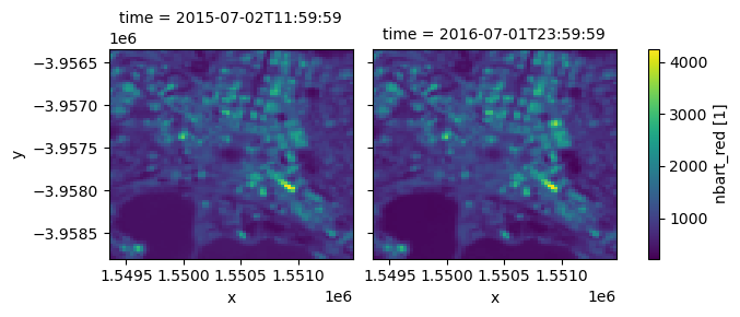

  geospatial_lon_units :

  degrees_east

We can now use this reloaded dataset just like the original dataset, for example by plotting one of its colour bands:

reloaded_ds.nbart_red.plot(col='time')

<xarray.plot.facetgrid.FacetGrid at 0x7f51a71a8520>

Clean-up

To remove the saved NetCDF file that we created, run the cell below. This is optional.

! rm output_netcdf.nc

---

Additional information

License: The code in this notebook is licensed under the Apache License, Version 2.0. Digital Earth Australia data is licensed under the Creative Commons by Attribution 4.0 license.

Contact: If you need assistance, please post a question on the Open Data Cube Slack channel or on the GIS Stack Exchange using the open-data-cube tag (you can view previously asked questions here). If you would like to report an issue with this notebook, you can file one on GitHub.

Last modified: June 2024

Compatible datacube version:

print(datacube.__version__)

1.8.18

Tags

Tags: sandbox compatible, NCI compatible, annual geomedian, NetCDF, write_dataset_to_netcdf, exporting data, metadata, shell commands