Modelling tides for coastal satellite data analysis 
Sign up to the DEA Sandbox to run this notebook interactively from a browser
Compatibility: Notebook currently compatible with the
DEA Sandboxenvironment onlyProducts used: ga_ls8c_ard_3
Background
Ocean tides are the periodic rise and fall of the ocean caused by the gravitational pull of the moon and sun and the earth’s rotation. Tides in coastal areas can greatly influence how these environments appear in satellite imagery as water levels vary by up to 12 metres (e.g. in north-western Australia). To be able to study coastal environments and processes along Australia’s coastline, it is vital to obtain data on tidal conditions at the exact moment each satellite image was acquired.
Description
This notebook demonstrates how to combine remotely sensed imagery with information about ocean tides using functions from the eo-tides Python package, allowing us to analyse satellite imagery by tide heights and tidal stage (e.g. low, high, ebb, flow). These functions use the global ocean tide models to calculate the height (relative to mean sea level) and stage of the tide at the exact moment each satellite image was acquired.
These tide modelling tools and tide models underpin DEA products including DEA Coastlines and DEA Intertidal.
The notebook demonstrates how to:
Model tide heights for specific coordinates and times using the
model_tidesfunctionModel tide heights for each satellite observation using the
tidal_tagfunctionCompute ebb or flow tide phase data to determine whether water levels were rising or falling in each satellite observation
Advanced: Spatially model tides into each pixel of a satellite dataset using
pixel_tidesAdvanced: Evaluate potential biases in the tides observed by a satellite using
tide_stats
Getting started
To run this analysis, run all the cells in the notebook, starting with the “Load packages” cell.
Load packages
[1]:
import datacube
import xarray as xr
import pandas as pd
import matplotlib.pyplot as plt
from datacube.utils.masking import mask_invalid_data
from eo_tides.utils import list_models
from eo_tides.model import model_tides
from eo_tides.eo import tag_tides, pixel_tides
from eo_tides.stats import tide_stats

import sys

sys.path.insert(1, "../Tools/")
from dea_tools.datahandling import load_ard
from dea_tools.plotting import rgb, display_map
Connect to the datacube
[2]:
dc = datacube.Datacube(app="Tidal_modelling")
Tide modelling directory
As a first step, we need to tell eo-tides the location of our tide model directory (if you are working off the DEA Sandbox, you will need to set this up using the setup instructions here).
We will pass this path to eo-tides functions using the directory parameter.
[3]:
directory = "/var/share/tide_models/"
We can use the `eo_tides.utils.list_models <../../api/#eo_tides.utils.list_models>`__ function to verify that we have tide model data available in this directory:
[4]:
list_models(directory=directory, show_supported=False);
────────────────────────────────────────────────────────────────────────────────
🌊 | Model | Expected path
────────────────────────────────────────────────────────────────────────────────
✅ │ EOT20 │ /var/share/tide_models/EOT20/ocean_tides
✅ │ FES2012 │ /var/share/tide_models/fes2012/data
✅ │ FES2014 │ /var/share/tide_models/fes2014/ocean_tide
✅ │ FES2014_extrapolated │ /var/share/tide_models/fes2014/ocean_tide_extrapolated
✅ │ FES2022 │ /var/share/tide_models/fes2022b/ocean_tide_20241025
✅ │ FES2022_extrapolated │ /var/share/tide_models/fes2022b/ocean_tide_extrapolated
✅ │ GOT4.10 │ /var/share/tide_models/GOT4.10c/grids_oceantide
✅ │ GOT5.5 │ /var/share/tide_models/GOT5.5/ocean_tides
✅ │ GOT5.5_extrapolated │ /var/share/tide_models/GOT5.5/extrapolated
✅ │ GOT5.6 │ /var/share/tide_models/GOT5.6/ocean_tides
✅ │ GOT5.6_extrapolated │ /var/share/tide_models/GOT5.6/extrapolated
✅ │ HAMTIDE11 │ /var/share/tide_models/hamtide
✅ │ TPXO10-atlas-v2-nc │ /var/share/tide_models/TPXO10_atlas_v2
✅ │ TPXO8-atlas-nc │ /var/share/tide_models/TPXO8_atlas_v1
✅ │ TPXO9-atlas-v5-nc │ /var/share/tide_models/TPXO9_atlas_v5
────────────────────────────────────────────────────────────────────────────────
Summary:
Available models: 15/52
Modelling tide heights using model_tides
In the example below, we use the `model_tides <../../api/#eo_tides.model.model_tides>`__ function to model hourly tides for the city of Broome, Western Australia across January 2018.
We will use the Finite Element Solution 2014 (FES2014) tidal model from the list of available models above.
Tip: To learn more about the science of tide prediction, refer to pyTMD Background Documentation and Glossary.
[5]:
# Model tides for a specific location and time period
tide_df = model_tides(
    x=122.2186,
    y=-18.0008,
    time=pd.date_range(start="2018-01-01", end="2018-01-31", freq="1h"),
    model="FES2014",
    directory=directory,
)

# Print outputs
tide_df.head()
Modelling tides with FES2014
[5]:
| tide_model | tide_height | |||
|---|---|---|---|---|
| time | x | y | ||
| 2018-01-01 00:00:00 | 122.2186 | -18.0008 | FES2014 | 1.280840 |
| 2018-01-01 01:00:00 | 122.2186 | -18.0008 | FES2014 | 2.356589 |
| 2018-01-01 02:00:00 | 122.2186 | -18.0008 | FES2014 | 2.571607 |
| 2018-01-01 03:00:00 | 122.2186 | -18.0008 | FES2014 | 2.036552 |
| 2018-01-01 04:00:00 | 122.2186 | -18.0008 | FES2014 | 1.129344 |
The resulting pandas.DataFrame contains:
time,x,y: Our original input timesteps and coordinatestide_model: a column listing the tide model usedtide_height: modelled tide heights representing tide height in metres relative to Mean Sea Level
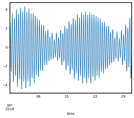
We can plot our modelled outputs to view how tides changed across the month. Looking at the y-axis, we can see that tides at this macrotidal region ranged from -4 metres up to a maximum of +4 metres relative to Mean Sea Level:
[6]:
tide_df.droplevel(["x", "y"]).tide_height.plot();
“One-to-many” and “one-to-one” modes
By default, the model_tides function operates in “one-to-many” mode, which will model tides at every requested location, for every requested timestep. This is particularly useful for satellite Earth observation applications where we may want to model tides for every satellite acquisition through time, for a large set of satellite pixels.
For example, if we provide two locations and two timesteps, the function will return four modelled tides:
2 locations * 2 timesteps = 4 modelled tides
[7]:
model_tides(
    x=[122.21, 122.22],
    y=[-18.20, -18.21],
    time=pd.date_range(start="2018-01-01", end="2018-01-31", periods=2),
    model="FES2014",
    directory=directory,
    mode="one-to-many",
)
Modelling tides with FES2014
[7]:
| tide_model | tide_height | |||
|---|---|---|---|---|
| time | x | y | ||
| 2018-01-01 | 122.21 | -18.20 | FES2014 | 1.263798 |
| 2018-01-31 | 122.21 | -18.20 | FES2014 | 0.267012 |
| 2018-01-01 | 122.22 | -18.21 | FES2014 | 1.265486 |
| 2018-01-31 | 122.22 | -18.21 | FES2014 | 0.260789 |
However, another common use case is having a list of locations you want to use to model tides for, each with a single timestep. Using “one-to-one” mode, we can model tides for each pair of locations and times:
2 timesteps at 2 locations = 2 modelled tides
For example, you may have a pandas.DataFrame containing x, y and time values:
[8]:
tide_df = pd.DataFrame({
    "time": pd.date_range(start="2018-01-01", end="2018-01-31", periods=2),
    "x": [122.21, 122.22],
    "y": [-18.20, -18.21],
})
tide_df
[8]:
| time | x | y | |
|---|---|---|---|
| 0 | 2018-01-01 | 122.21 | -18.20 |
| 1 | 2018-01-31 | 122.22 | -18.21 |
We can pass these values to model_tides directly, and run the function in “one-to-one” mode to return a tide height for each row:
[9]:
# Model tides and add back into dataframe
tide_df["tide_height"] = model_tides(
    x=tide_df.x,
    y=tide_df.y,
    time=tide_df.time,
    model="FES2014",
    directory=directory,
    mode="one-to-one",
).tide_height.to_numpy()

# Print dataframe with added tide height data:
tide_df.head()
Modelling tides with FES2014
[9]:
| time | x | y | tide_height | |
|---|---|---|---|---|
| 0 | 2018-01-01 | 122.21 | -18.20 | 1.263798 |
| 1 | 2018-01-31 | 122.22 | -18.21 | 0.260789 |
Modelling tide heights for each satellite observation using tag_tides
Modelling tides for a known set of points and times is useful, but for coastal remote sensing analysis it is more useful to automatically model the height of the tide at the exact moment each satellite image was taken.
Combining satellite data with tide information can help sort and filter images by tide height, allowing us to learn more about how coastal environments respond to the effect of changing tides.
To demonstrate how this can be done, we first need to load a time series of satellite imagery.
Set up data query
First we set up a query to define the area, time period and other parameters required for loading data. In this example, we will load several years of Landsat 8 data for intertidal mud flats south of Broome in Western Australia. We load the 'nbart_red', 'nbart_green', 'nbart_blue' bands so that we can plot the data as true colour imagery.
Tip: The dask_chunks parameter allows us to use Dask to lazily load data rather than load data directly into memory, which can take a long time and large amounts of memory. Lazy loading can be a very useful approach for when you need to load large amounts of data without crashing your analysis. In coastal applications, it allows us to load (using either .compute() or by plotting our data) only a small subset of observations from our entire
time series (e.g. only low or high tide observations) without having to load the entire dataset into memory first, which can greatly decrease processing times.
For more information about using Dask, refer to the Parallel processing with Dask notebook.
[10]:
# Set up data load query
query = {
    "x": (122.15, 122.26),
    "y": (-18.14, -18.24),
    "time": ("2020-01", "2020-06"),
    "measurements": ["nbart_red", "nbart_green", "nbart_blue"],
    "group_by": "solar_day",
    "dask_chunks": {},
}
We can preview the area that we will load data for:
[11]:
display_map(x=query['x'], y=query['y'])
[11]:
Load satellite time-series
To obtain some satellite data to analyse, we use the load_ard function to import a time series of Landsat 8 observations as an xarray.Dataset. The input data does not need to be from Landsat: any remotely-sensed imagery with timestamps and spatial coordinates provide enough data to run the tidal model.
[12]:
# Load available data from Landsat 8
ds = load_ard(
    dc=dc,
    products=["ga_ls8c_ard_3"],
    mask_pixel_quality=False,
    cloud_cover=(0, 10),  # load only scenes with <10% cloud
    **query
)

# Set nodata to NaN and print output
ds = mask_invalid_data(ds)
ds
Finding datasets
    ga_ls8c_ard_3
Returning 13 time steps as a dask array
[12]:
<xarray.Dataset> Size: 26MB
Dimensions:      (time: 13, y: 398, x: 415)
Coordinates:
  * time         (time) datetime64[ns] 104B 2020-01-13T01:49:41.792637 ... 20...
  * y            (y) float64 3kB -1.977e+06 -1.977e+06 ... -1.989e+06 -1.989e+06
  * x            (x) float64 3kB -1.041e+06 -1.041e+06 ... -1.029e+06 -1.029e+06
    spatial_ref  int32 4B 3577
Data variables:
    nbart_red    (time, y, x) float32 9MB dask.array<chunksize=(1, 398, 415), meta=np.ndarray>
    nbart_green  (time, y, x) float32 9MB dask.array<chunksize=(1, 398, 415), meta=np.ndarray>
    nbart_blue   (time, y, x) float32 9MB dask.array<chunksize=(1, 398, 415), meta=np.ndarray>
Attributes:
    crs:           EPSG:3577
grid_mapping: spatial_ref“Tagging” each satellite image with tide height metadata
We can now pass our satellite dataset ds to the tag_tides function to model a tide for each timestep in our dataset.
The tag_tides function uses the time and date of acquisition and the geographic centroid of each satellite observation as inputs for the selected tide model (EOT20 by default). It returns an xarray.DataArray called tide_height, with a modelled tide for every timestep in our satellite dataset:
[13]:
tides_da = tag_tides(
    data=ds,
    model="FES2014",
    directory=directory,
)

# Print modelled tides
tides_da
Setting tide modelling location from dataset centroid: 122.20, -18.19
Modelling tides with FES2014
[13]:
<xarray.DataArray 'tide_height' (time: 13)> Size: 52B
array([ 0.45971325, -0.7647201 ,  1.6473612 ,  2.3520935 , -1.8361684 ,
        2.7323349 ,  3.3902636 ,  1.9045722 ,  1.3566643 ,  3.8081174 ,
       -1.3738025 ,  2.9900064 , -2.156948  ], dtype=float32)
Coordinates:
  * time        (time) datetime64[ns] 104B 2020-01-13T01:49:41.792637 ... 202...
tide_model <U7 28B 'FES2014'We can easily combine these modelled tides with our original satellite data for further analysis. The code below adds our modelled tides as a new tide_height variable under Data variables.
[14]:
ds["tide_height"] = tides_da
ds
[14]:
<xarray.Dataset> Size: 26MB
Dimensions:      (time: 13, y: 398, x: 415)
Coordinates:
  * time         (time) datetime64[ns] 104B 2020-01-13T01:49:41.792637 ... 20...
  * y            (y) float64 3kB -1.977e+06 -1.977e+06 ... -1.989e+06 -1.989e+06
  * x            (x) float64 3kB -1.041e+06 -1.041e+06 ... -1.029e+06 -1.029e+06
    spatial_ref  int32 4B 3577
    tide_model   <U7 28B 'FES2014'
Data variables:
    nbart_red    (time, y, x) float32 9MB dask.array<chunksize=(1, 398, 415), meta=np.ndarray>
    nbart_green  (time, y, x) float32 9MB dask.array<chunksize=(1, 398, 415), meta=np.ndarray>
    nbart_blue   (time, y, x) float32 9MB dask.array<chunksize=(1, 398, 415), meta=np.ndarray>
    tide_height  (time) float32 52B 0.4597 -0.7647 1.647 ... -1.374 2.99 -2.157
Attributes:
    crs:           EPSG:3577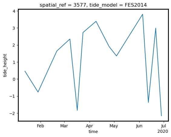
grid_mapping: spatial_refWe can plot this new tide_height variable over time to inspect the tide heights observed by the satellites in our time series:
[15]:
ds.tide_height.plot();
Example tide height analysis
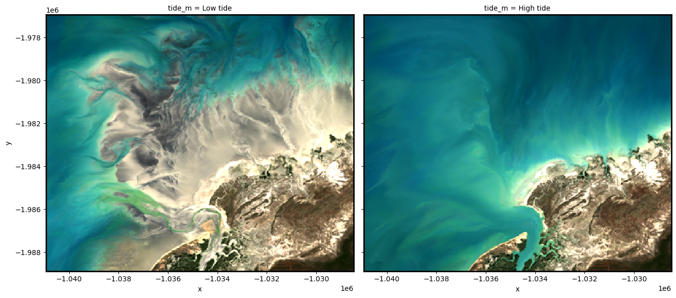
To demonstrate how tidally tagged images can be used to produce composites of high and low tide imagery, we can compute the lowest 20% and highest 20% of tide heights, and use these to filter our observations. We can then combine and plot these filtered observations to visualise how the landscape appears at low and high tide:
[16]:
# Calculate the lowest and highest 20% of tides
lowest_20, highest_20 = ds.tide_height.quantile([0.2, 0.8]).values

# Filter our data to low and high tide observations
filtered_low = ds.where(ds.tide_height <= lowest_20, drop=True)
filtered_high = ds.where(ds.tide_height >= highest_20, drop=True)

# Take the simple median of each set of low and high tide observations to
# produce a composite (alternatively, observations could be combined
# using a geomedian to keep band relationships consistent)
median_low = filtered_low.median(dim="time", keep_attrs=True)
median_high = filtered_high.median(dim="time", keep_attrs=True)

# Combine low and high tide medians into a single dataset and give
# each layer a meaningful name
ds_highlow = xr.concat([median_low, median_high], dim="tide_m")
ds_highlow["tide_m"] = ["Low tide", "High tide"]

# Plot low and high tide medians side-by-side
rgb(ds_highlow, col="tide_m")
/env/lib/python3.10/site-packages/rasterio/warp.py:387: NotGeoreferencedWarning: Dataset has no geotransform, gcps, or rpcs. The identity matrix will be returned.
  dest = _reproject(
Modelling ebb and flow tidal phases
The tag_tides function also allows us to determine whether each satellite observation was taken while the tide was rising/incoming (flow tide) or falling/outgoing (ebb tide) by setting return_phases=True. This is achieved by comparing tide heights 15 minutes before and after the observed satellite observation.
Ebb and flow data can provide valuable contextual information for interpreting satellite imagery, particularly in tidal flat or mangrove forest environments where water may remain in the landscape for considerable time after the tidal peak.
[17]:
tides_da = tag_tides(
    data=ds,
    model="FES2014",
    directory=directory,
    return_phases=True,
)

# Print modelled tides
tides_da
Setting tide modelling location from dataset centroid: 122.20, -18.19
Modelling tides with FES2014
Modelling tides with FES2014
[17]:
<xarray.Dataset> Size: 288B
Dimensions:      (time: 13)
Coordinates:
  * time         (time) datetime64[ns] 104B 2020-01-13T01:49:41.792637 ... 20...
    tide_model   <U7 28B 'FES2014'
Data variables:
    tide_height  (time) float32 52B 0.4597 -0.7647 1.647 ... -1.374 2.99 -2.157
tide_phase (time) object 104B 'high-flow' 'low-flow' ... 'low-flow'We now have data giving us the both the tide height and tidal phase (‘ebb’ or ‘flow’) for every satellite image:
[18]:
tides_da[["time", "tide_height", "tide_phase"]].to_dataframe()
[18]:
| tide_height | tide_phase | tide_model | |
|---|---|---|---|
| time | |||
| 2020-01-13 01:49:41.792637 | 0.459713 | high-flow | FES2014 |
| 2020-01-29 01:49:37.148233 | -0.764720 | low-flow | FES2014 |
| 2020-02-21 01:55:18.216005 | 1.647361 | high-flow | FES2014 |
| 2020-03-08 01:55:12.515274 | 2.352093 | high-flow | FES2014 |
| 2020-03-17 01:49:21.317513 | -1.836168 | low-flow | FES2014 |
| 2020-03-24 01:55:04.353944 | 2.732335 | high-flow | FES2014 |
| 2020-04-09 01:54:56.077227 | 3.390264 | high-flow | FES2014 |
| 2020-04-25 01:54:48.941936 | 1.904572 | high-flow | FES2014 |
| 2020-05-04 01:48:56.906589 | 1.356664 | high-ebb | FES2014 |
| 2020-06-05 01:49:03.396612 | 3.808117 | high-flow | FES2014 |
| 2020-06-12 01:54:54.641568 | -1.373803 | low-flow | FES2014 |
| 2020-06-21 01:49:12.757339 | 2.990006 | high-flow | FES2014 |
| 2020-06-28 01:55:03.091663 | -2.156948 | low-flow | FES2014 |
Advanced
Modelling tides for each pixel in a satellite time series using pixel_tides
The previous examples show how to model a single tide height for each satellite image using the centroid of the image as a tide modelling location. However, in reality tides vary spatially – potentially by several metres in areas of complex tidal dynamics. This means that an individual satellite image can capture a range of tide conditions.
We can use the pixel_tides function to capture this spatial variability in tide heights. For efficient processing, this function first models tides into a low resolution grid surrounding each satellite image in our time series. This lower resolution data includes a buffer around the extent of our satellite data so that tides can be modelled seamlessly across analysis boundaries.
pixel_tides can be run the same way as tag_tides, passing our satellite dataset ds as an input:
[19]:
# Model tides spatially
tides_lowres = pixel_tides(
    data=ds,
    resample=False,
    model="FES2014",
    directory=directory,
)

# Inspect output
tides_lowres
Creating reduced resolution 5000 x 5000 metre tide modelling array
Modelling tides with FES2014
Returning low resolution tide array
[19]:
<xarray.DataArray 'tide_height' (time: 13, y: 9, x: 8)> Size: 4kB
array([[[ 0.57769156, 0.55415046, 0.5259161 , 0.49562916,
0.47633326, 0.46905524, 0.4672558 , 0.4709148 ],
[ 0.56526524, 0.5388823 , 0.509618 , 0.47974148,
0.46539766, 0.45964727, 0.45893466, 0.46092138],
[ 0.55498874, 0.5268222 , 0.49733633, 0.47048044,
0.45847645, 0.45384654, 0.45487466, 0.45993322],
[ 0.5465381 , 0.5176067 , 0.4884161 , 0.46570984,
0.4551768 , 0.45085412, 0.45124668, 0.45960915],
[ 0.5387732 , 0.5113937 , 0.48358077, 0.4634806 ,
0.4526239 , 0.4526239 , 0.4526239 , 0.45960915],
[ 0.5303047 , 0.50673705, 0.48391014, 0.46635216,
0.46288854, 0.4526239 , 0.4526239 , 0.45960915],
[ 0.52317846, 0.50383574, 0.48635793, 0.46288854,
0.46288854, 0.46288854, 0.4526239 , 0.4526239 ],
[ 0.5201231 , 0.5035646 , 0.48875105, 0.48875105,
0.46288854, 0.46288854, 0.46288854, 0.4526239 ],
[ 0.5232942 , 0.5144136 , 0.48875105, 0.48875105,
0.48875105, 0.46288854, 0.46288854, 0.46288854]],
[[-0.60603726, -0.63949406, -0.677719 , -0.7166267 ,
...
[[-1.9688007 , -2.0175688 , -2.0648415 , -2.1072505 ,
-2.1397288 , -2.1613173 , -2.1760287 , -2.1816366 ],
[-1.9974343 , -2.0452147 , -2.0887754 , -2.1266108 ,
-2.1528528 , -2.1716719 , -2.184639 , -2.1922793 ],
[-2.0201716 , -2.0662994 , -2.106773 , -2.1395118 ,
-2.1611793 , -2.1772473 , -2.1881962 , -2.1943402 ],
[-2.0373454 , -2.081339 , -2.1195784 , -2.147655 ,
-2.165999 , -2.1728497 , -2.1882284 , -2.1951518 ],
[-2.0490637 , -2.0902984 , -2.1267738 , -2.1521003 ,
-2.174099 , -2.174099 , -2.174099 , -2.1951518 ],
[-2.0587957 , -2.095253 , -2.1274402 , -2.1504045 ,
-2.1559525 , -2.174099 , -2.174099 , -2.1951518 ],
[-2.0666773 , -2.0977893 , -2.124662 , -2.1559525 ,
-2.1559525 , -2.1559525 , -2.174099 , -2.174099 ],
[-2.0719645 , -2.0981443 , -2.1213965 , -2.1213965 ,
-2.1559525 , -2.1559525 , -2.1559525 , -2.174099 ],
[-2.071611 , -2.088035 , -2.1213965 , -2.1213965 ,
-2.1213965 , -2.1559525 , -2.1559525 , -2.1559525 ]]],
dtype=float32)
Coordinates:
* time (time) datetime64[ns] 104B 2020-01-13T01:49:41.792637 ... 20...
* x (x) float64 64B -1.052e+06 -1.048e+06 ... -1.022e+06 -1.018e+06
* y (y) float64 72B -1.962e+06 -1.968e+06 ... -1.998e+06 -2.002e+06
tide_model <U7 28B 'FES2014'
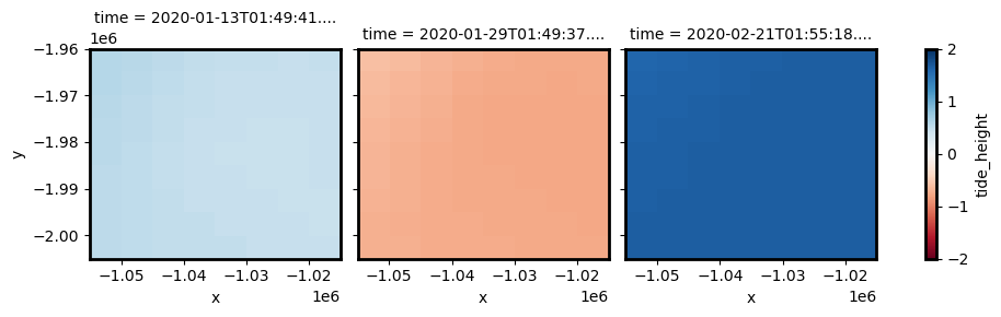
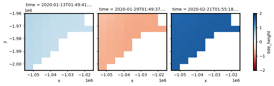
spatial_ref int32 4B 3577If we plot the resulting data, we can see that we now have two-dimensional tide surfaces for each timestep in our data (instead of the single tide height per timestamp returned by the tag_tides function).
Red below indicates low tide pixels, while blue indicates high tide pixels. If you look closely, you may see some spatial variability in tide heights within each timestep, with slight variations in tide heights along the north-west side of the study area:
[20]:
# Plot the first three timesteps in our data
tides_lowres.isel(time=[0, 1, 2]).plot.imshow(col="time", vmin=-2, vmax=2, cmap="RdBu")
[20]:
<xarray.plot.facetgrid.FacetGrid at 0x7fa331bd7f10>
Extrapolation
You may notice that modelled tides cover the entire 2D spatial extent of our images, even though the eastern side of our study area is land. This is because by default, eo-tides will extrapolate tide values into every pixel using nearest neighbour interpolation. This ensures every coastal pixel is allocated a tide height, but can produce inaccurate results the further a pixel is located from the ocean.
To turn off extrapolation, pass extrapolate=False:
[21]:
# Model tides spatially
tides_lowres = pixel_tides(
    data=ds,
    resample=False,
    extrapolate=False,
    model="FES2014",
    directory=directory,
)

# Plot the first four timesteps in our data
tides_lowres.isel(time=[0, 1, 2]).plot.imshow(col="time", vmin=-2, vmax=2, cmap="RdBu")
Creating reduced resolution 5000 x 5000 metre tide modelling array
Modelling tides with FES2014
Returning low resolution tide array
[21]:
<xarray.plot.facetgrid.FacetGrid at 0x7fa331bd5120>
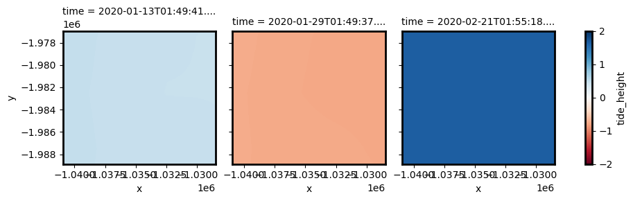
Reprojecting into original high-resolution spatial grid
By setting resample=True, we can use interpolation to re-project our low resolution tide data back into the resolution of our satellite image, resulting in an individual tide height for every pixel in our dataset through time and space:
[22]:
# Model tides spatially
tides_highres = pixel_tides(
    data=ds,
    resample=True,
    model="FES2014",
    directory=directory,
)

# Plot the first four timesteps in our data
tides_highres.isel(time=[0, 1, 2]).plot.imshow(col="time", vmin=-2, vmax=2, cmap="RdBu")
Creating reduced resolution 5000 x 5000 metre tide modelling array
Modelling tides with FES2014
Reprojecting tides into original resolution
[22]:
<xarray.plot.facetgrid.FacetGrid at 0x7fa331a38b20>
tides_highres will have exactly the same dimensions as ds, with a unique tide height for every satellite pixel:
[23]:
print(f"x: {len(ds.x)}, y: {len(ds.y)}, time: {len(ds.time)}")
x: 415, y: 398, time: 13
[24]:
print(f"x: {len(tides_highres.x)}, y: {len(tides_highres.y)}, time: {len(tides_highres.time)}")
x: 415, y: 398, time: 13
Because of this, our stack of tides can be added as an additional 3D variable in our dataset:
[25]:
ds["tide_height"] = tides_highres
ds
[25]:
<xarray.Dataset> Size: 34MB
Dimensions:      (time: 13, y: 398, x: 415)
Coordinates:
  * time         (time) datetime64[ns] 104B 2020-01-13T01:49:41.792637 ... 20...
  * y            (y) float64 3kB -1.977e+06 -1.977e+06 ... -1.989e+06 -1.989e+06
  * x            (x) float64 3kB -1.041e+06 -1.041e+06 ... -1.029e+06 -1.029e+06
    spatial_ref  int32 4B 3577
    tide_model   <U7 28B 'FES2014'
Data variables:
    nbart_red    (time, y, x) float32 9MB dask.array<chunksize=(1, 398, 415), meta=np.ndarray>
    nbart_green  (time, y, x) float32 9MB dask.array<chunksize=(1, 398, 415), meta=np.ndarray>
    nbart_blue   (time, y, x) float32 9MB dask.array<chunksize=(1, 398, 415), meta=np.ndarray>
    tide_height  (time, y, x) float32 9MB 0.4821 0.482 0.4818 ... -2.166 -2.166
Attributes:
    crs:           EPSG:3577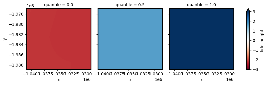
grid_mapping: spatial_refCalculating min/max/median/quantiles of tide heights for each pixel
Min, max or any specific quantile of all tide heights observed over a region can be calculated for each pixel by passing in a list of quantiles/percentiles using the calculate_quantiles parameter.
This calculation is performed on the low resolution modelled tide data before reprojecting to higher resolution, so should be faster than calculating min/max/median tide at high resolution:
[26]:
# Model tides spatially
tides_highres_quantiles = pixel_tides(
    data=ds,
    calculate_quantiles=(0, 0.5, 1),
    model="FES2014",
    directory=directory,
)

# Plot tide height quantiles
tides_highres_quantiles.plot.imshow(col="quantile", vmin=-3, vmax=3, cmap="RdBu")
Creating reduced resolution 5000 x 5000 metre tide modelling array
Modelling tides with FES2014
Computing tide quantiles
Reprojecting tides into original resolution
[26]:
<xarray.plot.facetgrid.FacetGrid at 0x7fa331ba6140>
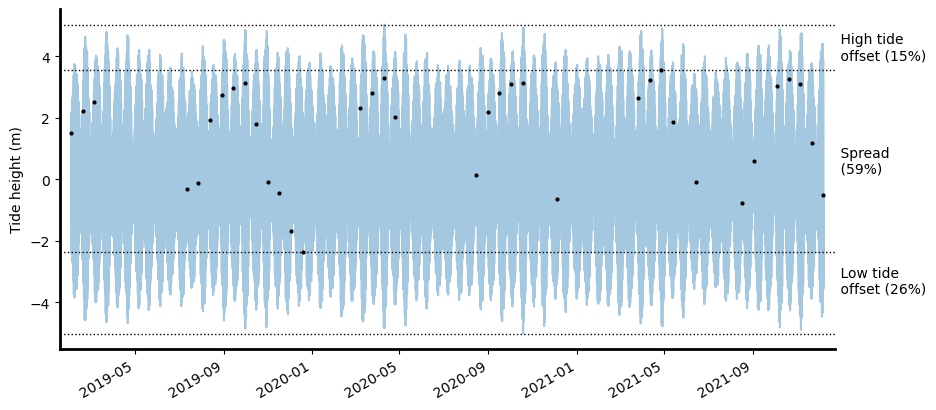
Evaluating tidal biases using tide_stats
Complex interactions between temporal tide dynamics and the regular overpass timing of sun-synchronous satellite sensors mean that satellites often do not always observe the entire tidal cycle. Biases in satellite coverage of the tidal cycle can mean that tidal extremes (e.g. the lowest or highest tides at a location) or particular tidal processes may either never be captured by satellites, or be over-represented in the satellite record. Local tide dynamics can cause these biases to vary greatly both through time and space, making it challenging to compare coastal processes consistently - particularly for large-scale coastal EO analyses.
To ensure that coastal EO analyses are not inadvertently affected by tide biases, it is important to compare how well the tides observed by satellites match the full range of tides at a location. The tidal_stats function compares the subset of tides observed by satellite data against the full range of tides modelled at a regular interval through time across the entire time period covered by the satellite dataset. This comparison is used to calculate several useful statistics and plots that
summarise how well your satellite data capture real-world tidal conditions.
Tip: For more information about the issue of tidal bias in sun-synchronous satellite observations of the coastline, refer to the eo-tides Calculating tide statistics and satellite biases guide.
[27]:
out_stats = tide_stats(
    data=ds,
    model="FES2014",
    directory=directory,
)
Using tide modelling location: 122.20, -18.19
Modelling tides with FES2014
Using tide modelling location: 122.20, -18.19
Modelling tides with FES2014


🌊 Modelled astronomical tide range: 9.75 m (-4.84 to 4.91 m).
🛰️ Observed tide range: 5.97 m (-2.16 to 3.81 m).

🔴 61% of the modelled astronomical tide range was observed at this location.
🟡 The highest 11% (1.11 m) of the tide range was never observed.
🔴 The lowest 27% (2.68 m) of the tide range was never observed.

🌊 Mean modelled astronomical tide height: 0.00 m.
🛰️ Mean observed tide height: 1.12 m.
⬆️ The mean observed tide height was 1.12 m higher than the mean modelled astronomical tide height.
The tide_stats function also outputs a pandas.Series object containing statistics for the results above, including:
mot: mean tide height observed by the satellite (metres)mat: mean modelled astronomical tide height (metres)hot: maximum tide height observed by the satellite (metres)hat: maximum tide height from modelled astronomical tidal range (metres)lot: minimum tide height observed by the satellite (metres)lat: minimum tide height from modelled astronomical tidal range (metres)otr: tidal range observed by the satellite (metres)tr: modelled astronomical tide range (metres)spread: proportion of the full modelled tidal range observed by the satelliteoffset_low: proportion of the lowest tides never observed by the satelliteoffset_high: proportion of the highest tides never observed by the satellitey: latitude used for modelling tide heightsx: longitude used for modelling tide heights
[28]:
out_stats
[28]:
mot              1.116000
mat              0.001000
hot              3.808000
hat              4.915000
lot             -2.157000
lat             -4.836000
otr              5.965000
tr               9.751000
spread           0.612000
offset_low       0.275000
offset_high      0.113000
x              122.205002
y              -18.190001
dtype: float32
Additional information
eo-tides documentation: For more detailed information about eo-tides functions and capabilities including tutorials and case study examples, refer to the official eo-tides Python package documentation.
FES2014: Tidal modelling is provided by the FES2014 global tidal model, implemented using functions from the pyTMD Python package. FES2014 was produced by NOVELTIS, LEGOS, CLS Space Oceanography Division and CNES. It is distributed by AVISO, with support from CNES (https://www.aviso.altimetry.fr/en/data/products/auxiliary-products/global-tide-fes/description-fes2014.html).
License: The code in this notebook is licensed under the Apache License, Version 2.0. Digital Earth Australia data is licensed under the Creative Commons by Attribution 4.0 license.
Contact: If you need assistance, please post a question on the Open Data Cube Discord chat or on the GIS Stack Exchange using the open-data-cube tag (you can view previously asked questions here). If you would like to report an issue with this notebook, you can file one on
GitHub.
Last modified: July 2025
Compatible datacube version:
[29]:
print(datacube.__version__)
1.8.19
Tags
Tags: sandbox compatible, NCI compatible, landsat 8, display_map, load_ard, rgb, tag_tides, tide_stats, model_tides, pixel_tides, tide modelling, intertidal, Dask, lazy loading